Experiment 7: Integration Grids

The argon dimer, and wiggles that shouldn’t be there

How the numerical integration grid affects DFT results, studied on the Ar2 dissociation curve.

At a glance. 31 Ar₂ distances plus the Ar atom, five functionals, three grids, all with def2-TZVP: 480 jobs. SG-1 jobs take seconds, SG-2 and SG-3 jobs a few minutes each, so plan your submissions. You will learn what the integration grid is, why meta-GGAs are sensitive to it, and how to choose a grid you can trust.

Warm-up

Loading the concept check…

Background

This experiment looks at a subtle issue that can affect the results of any exchange–correlation functional. Kohn–Sham (KS) DFT  [1,2] needs a real-space grid to evaluate the exchange–correlation integrals. Most programs build it with an algorithm Becke introduced in 1988  [3]: the integrals become weighted sums over a finite number of points arranged on spheres around each atom. A grid’s “density” is described by its number of radial shells and angular points per shell; (75,302), for example, means 75 radial shells with 302 points each. The choice of grid can change the results significantly, as Wheeler and Houk showed for the M06 family  [4,5] and Mardirossian and Head-Gordon for two generations of Minnesota functionals  [6,7]. They also point out that meta-GGA functionals usually need finer grids than GGAs.

Choosing the grid is often overlooked, and many practitioners are unaware of the issue. Relying on a program’s defaults is not a good idea, even though some programs pick the grid according to the functional  [8]. In this experiment you will study the dissociation curve of the argon dimer. The geometries come from the RG10 subset  [9] of the MGCDB84 database  [10], with the Ar–Ar distance between 3.0 and 6.0 Å. The interaction energy at each distance is

\[ \Delta E(r) = E\big(\mathrm{Ar}_2(r)\big) - 2\,E(\mathrm{Ar}). \]

Table 1: Reference interaction energies (kcal/mol) of the argon dimer as a function of the Ar–Ar distance (Å).

r	ΔE	r	ΔE	r	ΔE
3.0	2.24	4.1	–0.23	5.1	–0.07
3.1	1.21	4.2	–0.21	5.2	–0.06
3.2	0.57	4.3	–0.18	5.3	–0.05
3.3	0.18	4.4	–0.16	5.4	–0.05
3.4	–0.06	4.5	–0.14	5.5	–0.04
3.5	–0.19	4.6	–0.13	5.6	–0.04
3.6	–0.26	4.7	–0.11	5.7	–0.03
3.7	–0.28	4.8	–0.10	5.8	–0.03
3.8	–0.28	4.9	–0.09	5.9	–0.03
3.9	–0.27	5.0	–0.08	6.0	–0.02
4.0	–0.25

Use the functionals B3LYP  [11–15], M06-L  [16], M11  [17], M11-L  [18] and ωB97M-V  [19,20], and feel free to add others. Use the def2-TZVP basis set  [21] for all calculations, and try the grids SG-1, SG-2 and SG-3 (Q-Chem keyword XC_GRID = 1, 2 or 3).

Present your results as a dissociation curve like the one in Figure 1, which shows the VSXC functional  [22,23]. Before plotting, collect the data in a table like Table 2.

Figure 1: Behavior of the VSXC functional for the Ar dimer with different integration grids: SG-1 (orange), (75,302) (grey), (99,590) (green) and (175,974) (red). The reference curve is blue. Energy in kcal/mol, distance in Å.

Table 2: Data for the SG-1 curve in Figure 1 (VSXC functional; energy in kcal/mol, distance in Å).

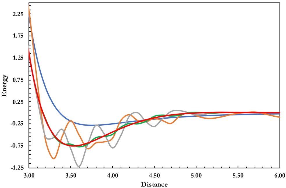
r	ΔE	r	ΔE	r	ΔE
3.0	2.33	4.1	–0.18	5.2	–0.12
3.1	0.71	4.2	–0.04	5.3	–0.09
3.2	–0.63	4.3	–0.17	5.4	–0.05
3.3	–1.04	4.4	–0.20	5.5	–0.01
3.4	–0.53	4.5	–0.13	5.6	0.01
3.5	–0.18	4.6	–0.18	5.7	0.02
3.6	–0.50	4.7	–0.24	5.8	–0.01
3.7	–0.81	4.8	–0.08	5.9	–0.06
3.8	–0.69	4.9	0.00	6.0	–0.10
3.9	–0.66	5.0	–0.06
4.0	–0.58	5.1	–0.12

What a grid looks like

Loading the grid explorer…

The molecules

Loading the molecules…

Predict first

Loading…

Run the calculations

This is the largest set of jobs of the course (5 functionals × 3 grids × 32 structures). SG-1 jobs take seconds, but the finer grids cost much more: expect a few minutes per job with SG-2 and SG-3. Work one functional and one grid at a time, and check the first curve before running the rest. Your instructor may split the functionals across the class.

Loading the job list…

Collect your results with a script

Reading 480 output files by hand is slow, and it’s easy to make mistakes. A small Python script does it for you: ⬇ extract_ex07.py. The same file works on macOS, Windows and Linux.

It reads every Q-Chem output file in a folder, including subfolders. It identifies each job from what Q-Chem echoed in the output (functional, XC_GRID, basis set and Ar–Ar distance), so your file names don’t matter. From each output it takes the total energy, the number of SCF cycles and the wall time, and writes them all to ex07_results.csv in the same folder. It only reads your outputs and never changes them.

Before you start: put all your Experiment 7 output files in one folder. Subfolders, such as one per grid, are fine.

macOS

1. Open Terminal (⌘-Space, type Terminal, Return).

2. Type python3 --version and press Return.

   • If you see Python 3.8 or newer, you’re ready.
   • If a window offers to install the command line developer tools, click Install, wait a few minutes, then try again.

3. Type python3 followed by a space. Drag extract_ex07.py from Finder into the Terminal window, type another space, then drag your outputs folder into the window. The line now looks like this:

   python3 /Users/you/Downloads/extract_ex07.py /Users/you/Documents/Ex7\ outputs

4. Press Return.

Windows

1. If you don’t have Python, install it from python.org/downloads. On the first screen of the installer, tick “Add python.exe to PATH”.

2. Open PowerShell (Start menu, type PowerShell, Enter).

3. Type py --version and press Enter. You should see Python 3.8 or newer. If PowerShell says py is not recognized, use python instead of py in the next step.

4. Type py followed by a space. Drag extract_ex07.py from File Explorer into the window, type another space, then drag your outputs folder into the window. The line now looks like this:

   py C:\Users\you\Downloads\extract_ex07.py "C:\Users\you\Documents\Ex7 outputs"

5. Press Enter.

Shortcut: if Python came from python.org, you can also double-click extract_ex07.py. A window opens and asks for the folder. Drag the folder into it and press Enter.

No Python (Colab)

If you can’t install Python on your computer, use Google Colab in the browser:

1. Zip your outputs folder (right-click → Compress on a Mac, Send to → Compressed (zipped) folder on Windows).

2. Open colab.research.google.com, create a new notebook, and upload the zip and extract_ex07.py with the folder icon on the left.

3. Run this in a cell. Replace outputs.zip with your zip’s name.

   !unzip -q outputs.zip -d outputs
   !python extract_ex07.py outputs

4. Download outputs/ex07_results.csv from the file panel (right-click → Download).

Read the report: don’t skip this step

The script prints a table with the number of usable jobs for each functional and grid. You need 32 in every cell, 480 in total. Then it lists:

• Missing jobs: run them.
• Problems: jobs that crashed or hit the 10-minute limit, SCF cycles that didn’t converge, a wrong basis set, or a missing XC_GRID (Q-Chem’s default grid depends on the version and the functional, so it doesn’t count as SG-1, SG-2 or SG-3). The script does not take any energy from these files. Fix the input, rerun the job, and run the script again.
• Jobs found more than once: the script uses the most recent good run. If it says the energies differ, find out why before you trust either one.
• Not recognized: other Q-Chem outputs in the folder (for example from another experiment). These are ignored.

You can run the script as often as you like. Each run rereads every output and rewrites the CSV.

WarningUse the script carefully

• Check its work. Open two or three output files, say one per grid, and compare the total energy, SCF cycles and wall time with the table below (Guide 3 shows where to find them). The script is a tool; the numbers you submit are your responsibility.
• Don’t edit the CSV and save it from Excel. Depending on your settings, Excel can round the energies or change commas into semicolons. You can look at it in Excel, but close it without saving, and import the file exactly as the script wrote it.
• Keep your output files. The CSV is a summary, not a replacement for them.

Enter your results

Record the total energy, SCF cycles and wall time of every job. The quickest way is ⬆ Import CSV below: choose ex07_results.csv and all three tabs fill in at once. If any cell already holds a different number, the page asks before replacing it. You can also type the values, or paste a column copied from a spreadsheet. The page computes all interaction energies ΔE(r) = E(Ar₂) − 2 E(Ar) for you and draws the curves as soon as one is complete.

Loading the results table…

Explore your data

The dashed black line is the reference curve. Wiggles that the reference doesn’t have are grid noise, not chemistry.

Loading…

Questions

Loading the questions…

Submit

Loading…

References

[1]

P. Hohenberg and W. Kohn, Phys. Rev. 136, B864 (1964).

[2]

W. Kohn and L. Sham, Phys. Rev. 140, A1133 (1965).

[3]

A. D. Becke, J. Chem. Phys. 88, 2547 (1988).

[4]

S. E. Wheeler and K. N. Houk, J. Chem. Theory Comput. 6, 395 (2010).

[5]

Y. Zhao and D. G. Truhlar, Theor. Chem. Acc. 120, 215 (2008).

[6]

N. Mardirossian and M. Head-Gordon, J. Chem. Theory Comput. 12, 4303 (2016).

[7]

N. Mardirossian and M. Head-Gordon, J. Chem. Theory Comput. 9, 4453 (2013).

[8]

Q-Chem, Inc., Q-Chem user’s manual: Numerical integration grids (XC_GRID), (n.d.).

[9]

K. T. Tang and J. P. Toennies, J. Chem. Phys. 118, 4976 (2003).

[10]

N. Mardirossian and M. Head-Gordon, Mol. Phys. 115, 2315 (2017).

[11]

S. H. Vosko, L. Wilk, and M. Nusair, Can. J. Phys. 58, 1200 (1980).

[12]

A. D. Becke, Phys. Rev. A 38, 3098 (1988).

[13]

C. Lee, W. Yang, and R. G. Parr, Phys. Rev. B 37, 785 (1988).

[14]

A. D. Becke, J. Chem. Phys. 98, 5648 (1993).

[15]

P. J. Stephens, F. J. Devlin, C. F. Chabalowski, and M. J. Frisch, J. Phys. Chem. 98, 11623 (1994).

[16]

Y. Zhao and D. G. Truhlar, J. Chem. Phys. 125, 194101 (2006).

[17]

R. Peverati and D. G. Truhlar, J. Phys. Chem. Lett. 2, 2810 (2011).

[18]

R. Peverati and D. G. Truhlar, J. Phys. Chem. Lett. 3, 117 (2012).

[19]

O. A. Vydrov and T. Van Voorhis, J. Chem. Phys. 133, 244103 (2010).

[20]

N. Mardirossian and M. Head-Gordon, J. Chem. Phys. 144, 214110 (2016).

[21]

F. Weigend and R. Ahlrichs, Phys. Chem. Chem. Phys. 7, 3297 (2005).

[22]

T. Van Voorhis and G. E. Scuseria, J. Chem. Phys. 109, 400 (1998).

[23]

T. Van Voorhis and G. E. Scuseria, J. Chem. Phys. 129, 219901 (2008).