7  Spin

Spin is a special property of particles that has no classical analogue. Spin is an intrinsic form of angular momentum carried by elementary particles, such as the electron.

7.1 Stern-Gerlach Experiment

In 1922, Otto Stern and Walter Gerlach performed an experiment that unintentionally led to the discovery that electrons have their own intrinsic angular momentum (spin), independent of their orbital motion in an atom. The experiment was done by putting a silver foil in an oven to vaporize its atoms. The silver atoms were collected into a beam that passed through an inhomogeneous magnetic field. The result was that the magnetic field split the beam into two (and only two) separate ones. The Stern–Gerlach experiment demonstrated that the spatial orientation of angular momentum is quantized into two components (up and down). Thus an atomic-scale system was shown to have intrinsically quantum properties. The experiment is normally conducted using electrically neutral particles such as silver atoms. This avoids the large deflection in the path of a charged particle moving through a magnetic field and allows spin-dependent effects to dominate. A schematic of the apparatus is shown in Fig. 7.1.

Figure 7.1: Schematic of the Stern–Gerlach experiment. A beam of silver atoms from an oven is collimated by two slits and passes between the poles of a magnet shaped to produce an inhomogeneous field. Right: the pattern on the screen expected for classical magnetic dipoles with random orientations (a continuous band) compared with the observed pattern (two separate spots).

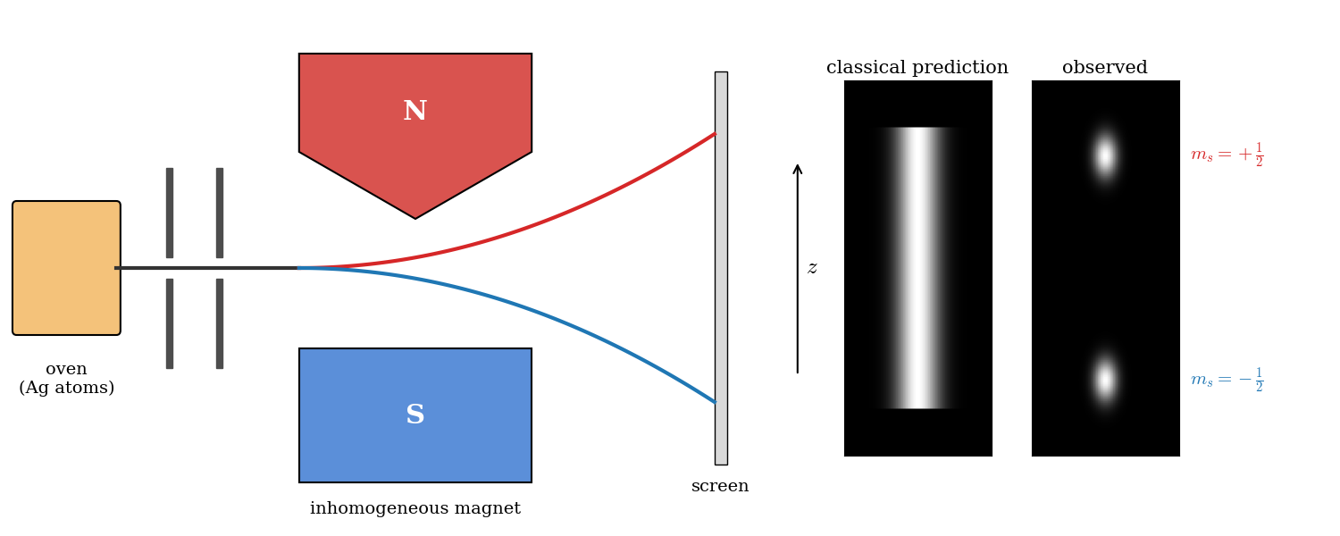
If the particle is treated as a classical spinning magnetic dipole, it will precess in a magnetic field because of the torque that the magnetic field exerts on the dipole. If it moves through a homogeneous magnetic field, the forces exerted on opposite ends of the dipole cancel each other out and the trajectory of the particle is unaffected. However, if the magnetic field is inhomogeneous then the force on one end of the dipole will be slightly greater than the opposing force on the other end, so that there is a net force which deflects the particle’s trajectory. If the particles were classical spinning objects, one would expect the distribution of their spin angular momentum vectors to be random and continuous. Each particle would be deflected by an amount proportional to its magnetic moment, producing some density distribution on the detector screen. Instead, the particles passing through the Stern–Gerlach apparatus are equally distributed among two possible values, with half of them ending up at an upper spot (“spin up”), and the other half at the lower spot (“spin down”). Since the particles are deflected by a magnetic field, spin is a magnetic property that is associated with some intrinsic form of angular momentum. As we saw in Chapter 6, the quantization of the angular momentum gives energy levels that are \((2\ell+1)\)-fold degenerate. Since along the direction of the magnet we observe only two possible eigenvalues for the spin, we conclude the following value for \(s\):

\[ 2s+1=2 \quad\Rightarrow\quad s=\frac{1}{2}. \tag{7.1}\]

The Stern-Gerlach experiment proves that electrons are spin-\(\frac{1}{2}\) particles. These have only two possible spin angular momentum values measured along any axis, \(+\frac {\hbar }{2}\) or \(-\frac {\hbar }{2}\), a purely quantum mechanical phenomenon. Because its value is always the same, it is regarded as an intrinsic property of electrons, and is sometimes known as “intrinsic angular momentum” (to distinguish it from orbital angular momentum, which can vary and depends on the presence of other particles).

The act of observing (measuring) the spin angular momentum along the \(z\) direction corresponds to the operator \(\hat{S}_z\), which projects the value of the total spin operator \(\hat{S}^2\) along the \(z\) axis. The eigenvalue equation for this projection operator is:

\[ \hat{S}_z \chi = \hbar m_s \chi, \tag{7.2}\]

where \(m_s=\left\{-s,+s\right\}=\left\{-\frac{1}{2},+\frac{1}{2}\right\}\) is the spin quantum number along the \(z\) component. The eigenvalues for the total spin operator \(\hat{S}^2\)—similarly to the angular momentum operator \(\hat{L}^2\) seen in Eq. 6.27—are:

\[ \hat{S}^2 \chi = \hbar^2 s(s+1) \chi, \tag{7.3}\]

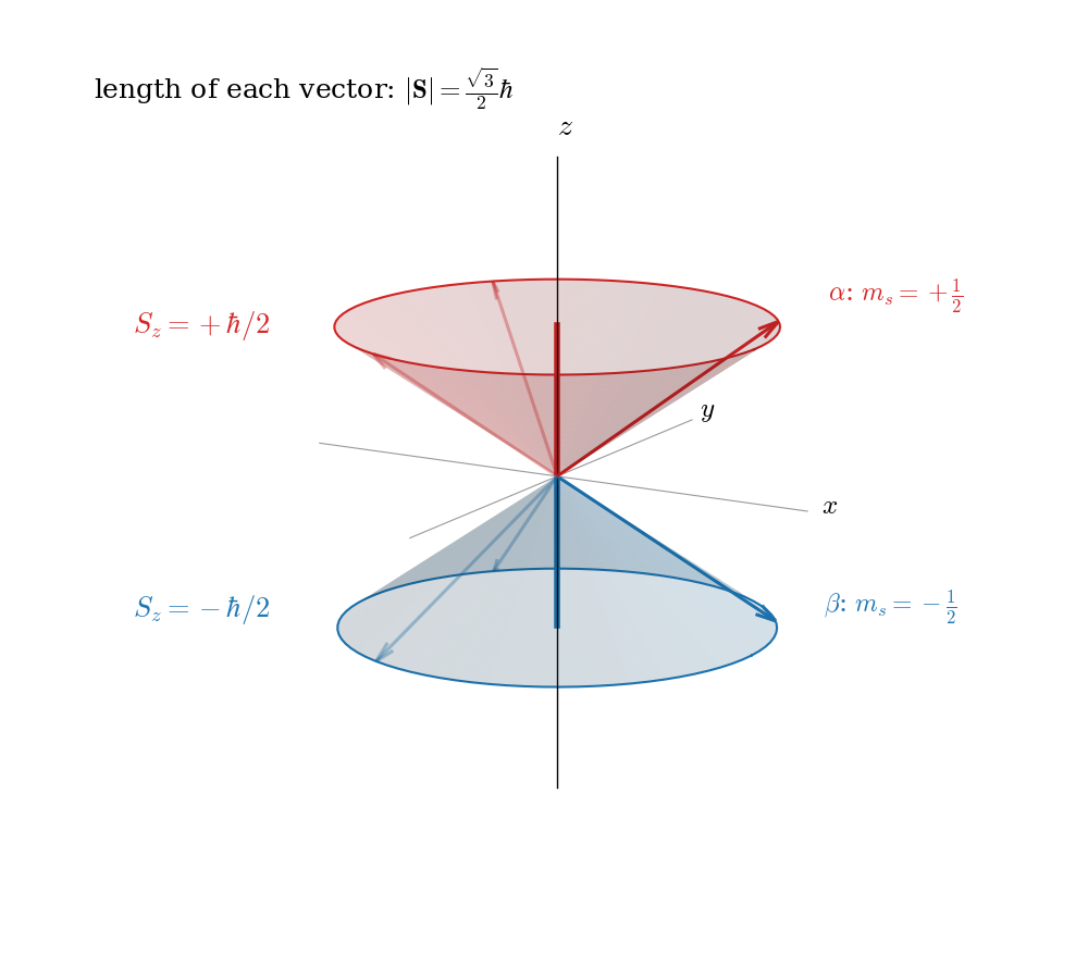
Notice that the magnitude of the spin angular momentum, \(|\mathbf{S}|=\hbar\sqrt{s(s+1)}=\frac{\sqrt{3}}{2}\hbar\approx0.87\hbar\), is larger than its largest possible projection on the \(z\) axis, \(\frac{1}{2}\hbar\). In other words, the spin vector can never point exactly along \(z\). A common way of picturing this result, shown in Fig. 7.2, is to imagine the spin vector lying somewhere on the surface of a cone around the \(z\) axis: its \(z\) component is well defined (\(+\frac{\hbar}{2}\) for \(\alpha\), and \(-\frac{\hbar}{2}\) for \(\beta\)), while its \(x\) and \(y\) components are not. As we will see in the next sections, this is a consequence of the fact that the three components of spin cannot be measured at the same time.

Figure 7.2: Vector model of the two spin states of an electron. The spin vector has length \(\frac{\sqrt{3}}{2}\hbar\) and a well-defined projection on the \(z\) axis, \(+\frac{\hbar}{2}\) (\(\alpha\), red) or \(-\frac{\hbar}{2}\) (\(\beta\), blue), but its direction around the cone (i.e., its \(x\) and \(y\) components) is undetermined. The lighter arrows show other possible orientations on the same cone.

The initial state of the particles in the Stern-Gerlach experiment is given by the following wave function:

\[ \chi = c_1\, \alpha + c_2 \,\beta, \tag{7.4}\]

where \(\alpha\) and \(\beta\) are the two eigenfunctions of \(\hat{S}_z\), corresponding to spin up (\(\uparrow\), \(m_s=+\frac{1}{2}\), eigenvalue \(+\frac{\hbar}{2}\)) and spin down (\(\downarrow\), \(m_s=-\frac{1}{2}\), eigenvalue \(-\frac{\hbar}{2}\)), respectively, and the coefficients \(c_1\) and \(c_2\) are complex numbers. The names \(\alpha\) and \(\beta\) for the two spin functions are standard in chemistry, and we will use them for the rest of this textbook. In this initial state, spin can point in any direction. The expectation value of the operator \(\hat{S}_z\) (the quantity that the Stern-Gerlach experiment measures), can be obtained using Eq. 6.20:

\[ \begin{aligned} <S_z> &= \int \chi^{*} \hat{S}_z \chi \, d\mathbf{s} \\ &= +\frac{\hbar}{2} \vert c_1\vert^2 -\frac{\hbar}{2} \vert c_2\vert^2, \end{aligned} \tag{7.5}\]

where the integration is performed along a special coordinate \(\mathbf{s}\) composed of only two values. Applying the normalization condition, Eq. 6.18, we can obtain:

\[ |c_{1}|^{2}+|c_{2}|^{2}=1 \quad\longrightarrow\quad |c_{1}|^{2}=|c_{2}|^{2}=\frac{1}{2}. \tag{7.6}\]

This equation is not sufficient to determine the values of the coefficients since they are complex numbers. Eq. 7.6, however, tells us that the squared magnitudes of the coefficients can be interpreted as probabilities of outcome from the experiment. This is true because their values are obtained from the normalization condition, and the normalization condition guarantees that the system is observed with probability equal to one. Summarizing, since we started with random initial directions, each of the two states, \(\alpha\) and \(\beta\), will be observed with equal probability of \(\frac{1}{2}\).

Example 7.1: Spin probabilities

An electron is described by the spin function \(\chi=\tfrac{\sqrt{3}}{2}\,\alpha+\tfrac{1}{2}\,\beta\). What are the probabilities of measuring spin up and spin down along \(z\), and what is \(\langle S_z\rangle\)?

Step 1: check the normalization. \(\left|\tfrac{\sqrt{3}}{2}\right|^2+\left|\tfrac{1}{2}\right|^2=\tfrac{3}{4}+\tfrac{1}{4}=1\).

Step 2: probabilities. \(P(\uparrow)=\tfrac{3}{4}\) and \(P(\downarrow)=\tfrac{1}{4}\).

Step 3: expectation value. Each result is weighted by its probability:

\[ \langle S_z\rangle=\tfrac{3}{4}\left(+\tfrac{\hbar}{2}\right)+\tfrac{1}{4}\left(-\tfrac{\hbar}{2}\right)=+\tfrac{\hbar}{4}. \]

As for any superposition, a single measurement gives either \(+\hbar/2\) or \(-\hbar/2\), never \(\hbar/4\).

7.2 Sequential Stern-Gerlach Experiments

An interesting result can be obtained if we link multiple Stern–Gerlach apparatuses into one experiment and we perform the measurement along two orthogonal directions in space. As we showed in the previous section, all particles leaving the first Stern-Gerlach apparatus are in an eigenstate of the \(\hat{S}_z\) operator (i.e., their spin is either “up” or “down” with respect to the \(z\)-direction). We can then take either one of the two resulting beams (for simplicity let’s take the “spin up” output), and perform another spin measurement on it. If the second measurement is also aligned along the \(z\)-direction then only one outcome will be measured, since all particles are already in the “spin up” eigenstate of \(\hat{S}_z\). In other words, the measurement of a particle being in an eigenstate of the corresponding operator leaves the state unchanged. The possible combinations of sequential experiments discussed in this section are summarized in Fig. 7.3.

Figure 7.3: Sequential Stern–Gerlach experiments, with the number of particles in each beam. (a) A single apparatus along \(z\) splits a beam of \(N\) particles into two equal beams. (b) A second apparatus along \(z\) does not split the spin-up beam any further. (c) An apparatus along \(x\) splits the spin-up beam into two beams, spin right and spin left; a third apparatus along \(z\) then splits the spin-right beam again into spin up and spin down, as if the first measurement had never happened.

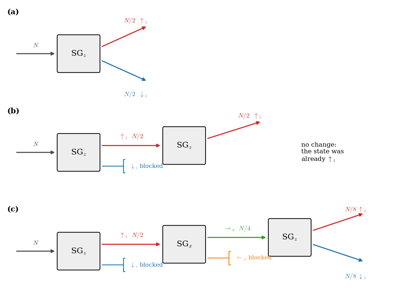
If, however, we perform the spin measurement along a direction perpendicular to the original \(z\)-axis (i.e., the \(x\)-axis) then the output will equally distribute among “spin up” or ”spin down” in the \(x\)-direction, which in order to avoid confusion, we can call “spin left” and “spin right”. Thus, even though we knew the state of the particles beforehand, in this case the measurement resulted in a random spin flip in either of the measurement directions. Mathematically, this property is expressed by the nonvanishing of the commutator of the spin operators:

\[ \left[\hat{S}_z,\hat{S}_x \right] \neq 0. \tag{7.7}\]

We can finally repeat the measurement a third time, with the magnet aligned along the original \(z\)-direction. According to classical physics, after the second apparatus, we would expect to have one beam with characteristic “spin up” and “spin left”, and another with characteristic “spin up” and “spin right”. The outcome of the third measurement along the original \(z\)-axis should be one output with characteristic “spin up”, regardless of which beam the magnet is applied (since the “spin down” component should have been “filtered out” by the first experiment, and the “spin left” and “spin right” component should be filtered out by the third magnet). This is not what is observed. The output of the third measurement is—once again—two beams in the \(z\) direction, one with “spin up” characteristic and the other with “spin down”.

This experiment shows that spin is not a classical property. The Stern-Gerlach apparatus does not behave as a simple filter, selecting beams with one specific pre-determined characteristic. The second measurement along the \(x\) axis destroys the previous determination of the angular momentum in the \(z\) direction. This means that this property cannot be measured on two perpendicular directions at the same time.

7.3 Spin Operators

The mathematics of quantum mechanics tells us that \(\hat{S}_z\) and \(\hat{S}_x\) do not commute. As we saw in Sec. 6.3.3, when two operators do not commute, in general there is no state in which both of the associated quantities have a definite value: they cannot be known at the same time.

In 3-dimensional space there are three directions that are orthogonal to each other \(\left\{x,y,z\right\}\). Thus, we can define a third spin projection operator along the \(y\) direction, \(\hat{S}_y\), corresponding to a new set of Stern-Gerlach experiments where the second magnet is oriented along a direction that is orthogonal to the two that we considered in the previous section. The total spin operator, \(\hat{S}^2\), can then be constructed similarly to the total angular momentum operator of Eq. 6.26, as:

\[ \begin{aligned} \hat{S}^2 &=\hat{S}\cdot\hat{S}=\left(\mathbf{i}\hat{S}_x+\mathbf{j}\hat{S}_y+\mathbf{k}\hat{S}_z\right)\cdot\left(\mathbf{i}\hat{S}_x+\mathbf{j}\hat{S}_y+\mathbf{k}\hat{S}_z \right) \\ &=\hat{S}_x^2+\hat{S}_y^2+\hat{S}_z^2, \end{aligned} \tag{7.8}\]

with \(\left\{\mathbf{i},\mathbf{j},\mathbf{k}\right\}\) the unit vectors in three-dimensional space.

Wolfgang Pauli explicitly derived the relationships between all three spin projection operators. Assuming the magnetic field along the \(z\) axis, Pauli’s relations can be written using simple equations involving the two possible eigenstates \(\alpha\) and \(\beta\):

\[ \begin{aligned} \hat{S}_x \alpha = \frac{\hbar}{2} \beta \qquad \hat{S}_y \alpha &= \frac{\hbar}{2} i \beta \qquad \hat{S}_z \alpha = \frac{\hbar}{2} \alpha \\ \hat{S}_x \beta = \frac{\hbar}{2} \alpha \qquad \hat{S}_y \beta &= - \frac{\hbar}{2} i \alpha \qquad \hat{S}_z \beta = -\frac{\hbar}{2} \beta, \end{aligned} \tag{7.9}\]

where \(i\) is the imaginary unit (\(i^2=-1\)). In other words, for \(\hat{S}_z\) we have eigenvalue equations, while the remaining components have the effect of permuting state \(\alpha\) with state \(\beta\) after multiplication by suitable constants. We can use these equations, together with Eq. 6.7, to calculate the commutator for each pair of spin projection operators:

\[ \begin{aligned} \left[\hat{S}_x, \hat{S}_y\right] &= i\hbar\hat{S}_z \\ \left[\hat{S}_y, \hat{S}_z\right] &= i\hbar\hat{S}_x \\ \left[\hat{S}_z, \hat{S}_x\right] &= i\hbar\hat{S}_y, \end{aligned} \tag{7.10}\]

In words: no two components of the spin commute with each other, so, as we saw for position and momentum, no state can have definite values of two different components at the same time. This is exactly what the sequential Stern–Gerlach experiments showed.

NoteProof: the commutators of the spin components

The commutators in Eq. 7.10 follow from Pauli’s relations, Eq. 7.9, and the definition of commutator, Eq. 6.7. We apply both sides to \(\alpha\) (applying them to \(\beta\) gives the same result). For the first pair:

\[ \begin{aligned} \left[\hat{S}_x, \hat{S}_y\right] \alpha &= \hat{S}_x\hat{S}_y\alpha-\hat{S}_y\hat{S}_x\alpha \\ &= \hat{S}_x \left(\frac{\hbar}{2}i \beta \right)-\hat{S}_y \left(\frac{\hbar}{2} \beta \right) \\ &= \frac{\hbar}{2}i \left(\frac{\hbar}{2} \alpha \right)- \frac{\hbar}{2} \left(-\frac{\hbar}{2}i \alpha \right) \\ &= \left(\frac{\hbar^2}{4}+\frac{\hbar^2}{4}\right)i\alpha \\ &= \frac{\hbar^2}{2}i \alpha \\ &= i\hbar\hat{S}_z \alpha \end{aligned} \tag{7.11}\]

7.4 Operators Commuting with the Hamiltonian

We have now met several quantum numbers: \(n\) for the particle in a box, \(m_\ell\) for the particle on a ring, \(\ell\) and \(m_\ell\) for the particle on a sphere, \(n\), \(\ell\), and \(m_\ell\) for the hydrogen atom, and now \(m_s\) for spin. At first sight, they look like a random collection of labels, each one coming out of a different calculation. To conclude this chapter, let’s step back and see that they all have the same origin.

The key is the theorem that we discussed in Sec. 6.3.3: if an operator \(\hat{A}\) commutes with the Hamiltonian, \([\hat{H},\hat{A}]=0\), we can find wave functions that are eigenfunctions of both. Each of these wave functions then has a definite energy and a definite value of the observable \(A\), and we can use the eigenvalue of \(\hat{A}\) as a label for the state. Moreover, since \(\hat{A}\) commutes with \(\hat{H}\), which controls the time evolution (Sec. 6.4), this label does not change in time: the observable \(A\) is conserved. Physicists call such a label a good quantum number.

So, the question “which quantum numbers does a system have?” becomes “which operators commute with its Hamiltonian?”. And, as we will see in the examples below, the answer to this second question comes from the symmetry of the system: every time the system looks the same after some operation (a shift, a reflection, a rotation), there is an operator that commutes with \(\hat{H}\), and a quantum number that comes with it.

7.4.1 Free particle: shifts and momentum

A free particle feels no potential, so its Hamiltonian contains only the kinetic energy, \(\hat{H}=\hat{p}^2/2m\). Its symmetry is that space looks the same everywhere: if we shift the whole system by any distance, nothing changes. The operator associated with this symmetry is the momentum, and since \(\hat{H}\) contains only \(\hat{p}\), the two commute:

\[ [\hat{H}, \hat{p}] = 0. \tag{7.12}\]

This is why the free-particle solutions of Chapter 3, the plane waves \(e^{ikx}\), have both a definite energy and a definite momentum, \(p=\hbar k\), and why we can label them with \(k\).

7.4.2 Particle in a box: no more momentum, but parity

Inside a box, the particle is still free, but the walls break the symmetry: if we shift the system, the walls move, and the problem changes. As a consequence, \(\hat{p}\) no longer commutes with \(\hat{H}\), and momentum is not a good quantum number. We can check this directly: the eigenfunctions of the particle in a box, \(\sin(n\pi x/a)\), are not eigenfunctions of \(\hat{p}=-i\hbar\frac{d}{dx}\), since the derivative turns a sine into a cosine. (Using Euler’s formula, each sine is a combination of two plane waves, one moving to the right and one to the left, with opposite momenta. A measurement of momentum would give either one, but the state does not have a definite momentum.)

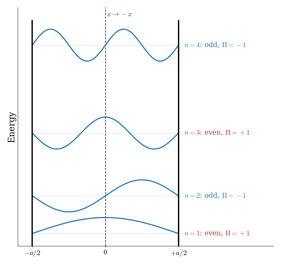
Some symmetry, however, survives. If we place the box symmetrically, between \(-a/2\) and \(+a/2\), the system looks the same when we reflect it through its center, \(x\rightarrow-x\). The operator that performs this reflection is called the parity operator, \(\hat{\Pi}\):

\[ \hat{\Pi}\,\psi(x) = \psi(-x). \tag{7.13}\]

Whenever the potential is symmetric, \(V(-x)=V(x)\), the Hamiltonian does not change under reflection, and it commutes with parity, \([\hat{H},\hat{\Pi}]=0\). The energy eigenfunctions can then be chosen to be eigenfunctions of parity too. Since reflecting twice brings us back to where we started, the only possible eigenvalues are \(+1\) and \(-1\):

• Even functions are unchanged by the reflection, \(\psi(-x)=+\psi(x)\).
• Odd functions change sign, \(\psi(-x)=-\psi(x)\).

As shown in Fig. 7.4, the states of the particle in a box alternate between even and odd as the energy increases. Parity is a simple label, but a very useful one: it is the origin of the \(g\) and \(u\) labels of molecular orbitals in Chapter 11, and of many selection rules in Chapter 13, since the integral of an odd function over a symmetric interval is zero (Sec. A.3).

Figure 7.4: The first four eigenfunctions of a particle in a box placed symmetrically between \(-a/2\) and \(+a/2\). Even states (red labels) are unchanged by the inversion \(x\rightarrow -x\) (reflection through the purple dashed line), and odd states (blue labels) change sign.

7.4.3 Particle on a ring and on a sphere: rotations and angular momentum

A particle on a ring looks the same if we rotate the ring by any angle around its axis, \(z\). The operator associated with rotations around \(z\) is the \(z\) component of the angular momentum, so:

\[ [\hat{H}, \hat{L}_z] = 0. \tag{7.14}\]

This is why the solutions of the particle on a ring, \(e^{im_\ell\phi}\), have both a definite energy and a definite angular momentum, \(L_z=m_\ell\hbar\) (Chapter 4), and why we can label them with \(m_\ell\).

A particle on a sphere looks the same after a rotation around any axis. Its Hamiltonian commutes with all three components of the angular momentum, and therefore also with \(\hat{L}^2\). Since the components do not commute with each other (Chapter 6), we cannot use all of them as labels at the same time. The best we can do is to pick \(\hat{L}^2\) and one component, by convention \(\hat{L}_z\):

\[ [\hat{H}, \hat{L}^2] = 0, \qquad [\hat{H}, \hat{L}_z] = 0, \tag{7.15}\]

which give the two quantum numbers \(\ell\) (from \(L^2=\hbar^2\ell(\ell+1)\)) and \(m_\ell\) (from \(L_z=\hbar m_\ell\)) of the spherical harmonics. There is one more consequence of the symmetry. Since the sphere has no preferred direction, the energy cannot depend on the orientation of the angular momentum, that is, on \(m_\ell\). This is why each level \(\ell\) is \((2\ell+1)\) times degenerate: the degeneracy is the rotational symmetry.

7.4.4 Hydrogen atom: one label more, and an extra degeneracy

The Coulomb potential of the hydrogen atom depends only on the distance from the nucleus, \(r\), so the atom has the same rotational symmetry as the sphere, and \(\hat{H}\) commutes with \(\hat{L}^2\) and \(\hat{L}_z\). Together with the energy itself, this gives the three labels \(n\), \(\ell\), and \(m_\ell\) of the hydrogen orbitals.

Rotational symmetry explains why the energy does not depend on \(m_\ell\). It does not explain, however, why the energy of hydrogen does not depend on \(\ell\) either, so that, for example, the \(2s\) and \(2p\) orbitals have the same energy (Chapter 5). This additional degeneracy is a special property of the \(1/r\) potential, which has a hidden symmetry that goes beyond simple rotations (its discussion is beyond the scope of this book). As soon as the potential is no longer exactly \(1/r\), as for an electron in a many-electron atom shielded by the others, this degeneracy disappears, and the \(2s\) and \(2p\) energies split (Chapter 9).

7.4.5 Spin: why it matters

The hydrogen Hamiltonian that we used does not contain spin at all, so it automatically commutes with \(\hat{S}^2\) and \(\hat{S}_z\). Each spatial state \((n,\ell,m_\ell)\) can therefore be combined with either spin function, \(\alpha\) or \(\beta\), giving a fourth label, \(m_s=\pm\frac{1}{2}\), and doubling the number of states. In hydrogen, spin does not change the energies (except for the tiny spin–orbit effects that we will discuss in Sec. 9.4), but it changes the counting: this is why the first shell of the periodic table holds two elements, and the second one eight.

In atoms with many electrons, the same reasoning applies to the whole atom. The atom as a whole is still rotationally symmetric, so the total orbital angular momentum, \(L\), and the total spin, \(S\), become the good quantum numbers that label its states. These are the labels of the term symbols that we will meet in Sec. 9.4.

To summarize, every quantum number we use in chemistry can be traced back to a symmetry of the system, as collected in Table 7.1.

Table 7.1: Symmetries, commuting operators, and quantum numbers.

System	Symmetry	Commutes with \(\hat{H}\)	Quantum numbers
Free particle	shifts in space	\(\hat{p}\)	\(k\)
Symmetric box	reflection \(x\rightarrow-x\)	\(\hat{\Pi}\)	parity (even/odd)
Particle on a ring	rotations around \(z\)	\(\hat{L}_z\)	\(m_\ell\)
Sphere, hydrogen atom	all rotations	\(\hat{L}^2\), \(\hat{L}_z\)	\(\ell\), \(m_\ell\)
Electron spin	(not in \(\hat{H}\))	\(\hat{S}^2\), \(\hat{S}_z\)	\(s\), \(m_s\)
Many-electron atom	all rotations	\(\hat{L}^2\), \(\hat{S}^2\) (total)	\(L\), \(S\)

7.5 Chapter Review

7.5.1 Key Ideas

• The Stern–Gerlach experiment shows that electrons have an intrinsic angular momentum, spin, with only two possible \(z\) components, \(\pm\hbar/2\).
• The spin components do not commute with each other, so measuring one of them randomizes the others.
• A spin state \(c_1\alpha+c_2\beta\) gives spin up with probability \(|c_1|^2\) and spin down with probability \(|c_2|^2\).
• Every quantum number comes from a symmetry of the system, through an operator that commutes with the Hamiltonian.
• Spin adds a fourth label, \(m_s\), and doubles the number of states of each orbital.

7.5.2 Study Questions

1. In the Stern–Gerlach experiment, a beam of silver atoms passing through an inhomogeneous magnetic field:

1. is deflected into a continuous band
2. is not deflected
3. splits into three beams
4. is absorbed by the magnet
5. splits into two beams

---

2. The possible results of a measurement of the \(z\) component of the spin of an electron are:

1. \(+\hbar\) and \(-\hbar\)
2. \(+\frac{\hbar}{2}\) and \(-\frac{\hbar}{2}\)
3. \(0\) and \(\hbar\)
4. any value between \(-\frac{\hbar}{2}\) and \(+\frac{\hbar}{2}\)
5. \(\frac{\sqrt{3}}{2}\hbar\)

---

3. The magnitude of the spin of an electron, \(\frac{\sqrt{3}}{2}\hbar\), is larger than its largest \(z\) component, \(\frac{\hbar}{2}\). This means that:

1. the spin always points along \(z\)
2. the measurement of \(S_z\) is wrong
3. the spin can never point exactly along the \(z\) axis
4. the electron has two spins
5. the spin is not quantized

---

4. An electron is described by the spin function \(c_1\alpha+c_2\beta\). The probability of measuring spin up along \(z\) is:

1. \(c_1\)
2. \(|c_2|^2\)
3. \(\frac{1}{2}\), whatever the coefficients
4. \(|c_1|^2\)
5. \(|c_1|^2+|c_2|^2\)

---

5. Electrons selected with spin up along \(z\) pass through an apparatus aligned along \(x\), and then the spin-up-along-\(x\) beam is measured again along \(z\). The result is:

1. both spin up and spin down along \(z\), with equal probability
2. only spin up along \(z\)
3. only spin down along \(z\)
4. no electrons
5. a continuous distribution of values

---

6. The commutator \([\hat{S}_x,\hat{S}_y]=i\hbar\hat{S}_z\neq0\) means that:

1. \(S_x\) and \(S_y\) are always zero
2. spin is a classical vector
3. the three spin components have the same value
4. an electron cannot have definite values of two different spin components at the same time
5. \(S_z\) cannot be measured

---

7. A quantum number is called a good quantum number when:

1. it is an eigenvalue of an operator that commutes with the Hamiltonian, so it does not change in time
2. it is an integer
3. it determines the energy
4. it is positive
5. it can only take two values

---

8. For a particle in a box placed symmetrically around \(x=0\), the energy eigenfunctions are:

1. all even
2. alternately even and odd under the reflection \(x\rightarrow-x\)
3. all odd
4. neither even nor odd
5. eigenfunctions of momentum

---

9. Why are the energy levels of a particle on a sphere \((2\ell+1)\) times degenerate?

1. because the Hamiltonian does not commute with \(\hat{L}_z\)
2. because of the Pauli exclusion principle
3. because the sphere has no preferred direction, so the energy cannot depend on \(m_\ell\)
4. because of spin
5. because the potential energy is \(1/r\)

---

10. Including spin, how many different states does the \(n=2\) level of the hydrogen atom have?

1. \(2\)
2. \(4\)
3. \(6\)
4. \(16\)
5. \(8\)

---

ExampleAnswers

1.e, 2.b, 3.c, 4.d, 5.a, 6.d, 7.a, 8.b, 9.c, 10.e