1  Brief Summary of Classical Physics

Quantum mechanics cannot be derived from classical physics, but it was built by physicists who knew classical physics very well, and many of its ideas and equations are borrowed from it. Before discussing, in the next chapter, the experiments that classical physics could not explain, we will review the classical concepts that we will need the most: the description of motion through forces and through energy, the electrostatic interaction between charged particles, and the physics of waves.

1.1 Classical Mechanics

1.1.1 Newtonian Formulation

Classical mechanics as formulated by Isaac Newton (1643–1727) is all about forces. Newtonian mechanics works well for problems where we know the forces and have a reasonable coordinate system. In these cases, the net force acting on a system at position \(\mathbf{r}\) in Cartesian 3-dimensional space \(\left\{ x,y,z \right\}\) is simply:

\[ F_{\mathrm{net}}(\mathbf{r}) = m\ddot{\mathbf{r}} = m \frac{d^2 \mathbf{r}}{dt^2}. \tag{1.1}\]

Or, in other words, if we know the net force acting on a system of mass \(m\) at position \(\mathbf{r}\) at some time \(t_0\), we can use Eq. 1.1 to calculate the position of the system at any future (or past) time. We have completely determined the dynamical evolution of the system.¹

Example 1.1: A ball tossed straight up (Newton)

A ball of mass \(m\) is at ground level and tossed straight up from an initial position \(x_0\) with an initial velocity \(\dot{x}_0\) and subject to gravity alone. Calculate the equation of motion for the ball (i.e. where is the ball going to be after some time \(t\)?).²

Solution: Since the only force acting on the ball is gravity, we can use the equation for the gravitational force to start our derivation:

\[ F_{\mathrm{gravity}}=-mg, \tag{1.2}\]

with \(g\) the gravitational acceleration (\(g=9.8\; \mathrm{m}/\mathrm{s}^{2}\)). We can then replace this expression into Eq. 1.1, to obtain:

\[ \begin{aligned} -mg &=m \ddot{\mathbf{r}} \\ -g &=\ddot{\mathbf{r}} \\ -g &=\frac{d\dot{\mathbf{r}}}{dt}. \\ \end{aligned} \tag{1.3}\]

Working in a 1-dimensional case, we can replace \(\mathbf{r}\) with position \(x\) to obtain:

\[ \begin{aligned} -mg &=m \ddot{x} \\ -g &=\ddot{x} \\ -g &=\frac{d\dot{x}}{dt}. \\ \end{aligned} \tag{1.4}\]

which can then be integrated with respect to time, to obtain:

\[ \begin{aligned} -g\int_{t=0}^{t} dt &=\int_{\dot{x}_0}^{\dot{x}} d\dot{x}\\ \dot{x} &= \dot{x}_0-gt\\ \frac{dx}{dt} &= \dot{x}_0-gt,\\ \end{aligned} \tag{1.5}\]

which can be further integrated with respect to time, to give:

\[ \begin{aligned} \int_{x_0}^{x} dx &= \int_{t=0}^{t} \dot{x}_0 dt -g \int_{t=0}^{t}tdt\\ x &= x_0 + \dot{x}_0 t -\frac{1}{2}gt^2. \end{aligned} \tag{1.6}\]

This final equation is the equation of motion for the ball, from which we can calculate the position of the ball at any time \(t\). Notice how the equation of motion does not depend on the mass of the ball!

Numerical problem: How much time will a ball ejected from a height of \(1 \;\mathrm{m}\) at an initial velocity of \(10 \;\mathrm{m/s}\) take to hit the floor?

We can use the equation of motion obtained above to solve this problem, and obtain for this specific case \(t\simeq2.14\;\mathrm{s}\).³

Newton’s equation is not the only way of writing the laws of classical mechanics. Physicists have developed other, equivalent formulations, which give exactly the same results but are more convenient for some problems. The most famous are the Lagrangian formulation, based on the difference between the kinetic and the potential energy of a system, and the Hamiltonian formulation, based on their sum.⁴ Only the second one will be important for us, because it is the one that quantum mechanics is built upon.

1.1.2 Hamiltonian Formulation

Newton’s mechanics is built around forces. Hamiltonian mechanics, instead, is built around energy. Its goal is to describe the motion of a system starting from a single function, the total energy, written in terms of where the particle is and how much momentum it has. This is exactly the starting point that we will use in quantum mechanics, which is why we need to get familiar with it now.

The first ingredient is the momentum of a particle of mass \(m\) moving with velocity \(\dot{x}\) (we will work in one dimension to keep things simple):

\[ p = m\dot{x}. \tag{1.7}\]

Momentum carries the same information as velocity, but, as we will see in the next chapter, it is the quantity that appears naturally when we describe particles in quantum mechanics.

The second ingredient is the total energy of the system, which is the sum of the kinetic energy, \(K\), and the potential energy, \(V\):

\[ H = K + V. \tag{1.8}\]

When we write this total energy as a function of the position, \(x\), and the momentum, \(p\), we call it the Hamiltonian of the system, and we use the symbol \(H\). Since the kinetic energy is \(K=\frac{1}{2}m\dot{x}^2\), and \(\dot{x}=p/m\), we can write \(K=\frac{p^2}{2m}\), and the Hamiltonian of a particle becomes:

\[ H(x,p) = \frac{p^2}{2m} + V(x). \tag{1.9}\]

This equation is the most important result of this section. The first term depends only on the momentum, and it is the same for every system. The second term depends only on the position, and it is what makes each system different: a ball in the gravitational field of the Earth, an electron attracted by a nucleus, or two atoms connected by a chemical bond differ only in their potential energy, \(V(x)\).

Once we know the Hamiltonian, the motion of the system can be obtained from two simple equations, called Hamilton’s equations:

\[ \begin{aligned} \dot{x}=\frac{dx}{dt} &= +\frac{\partial H}{\partial p}, \\ \dot{p}=\frac{dp}{dt} &= -\frac{\partial H}{\partial x}. \end{aligned} \tag{1.10}\]

These two equations are less mysterious than they look. If we apply them to Eq. 1.9, the first one gives \(\dot{x}=\frac{p}{m}\), which is just the definition of momentum, Eq. 1.7, read backwards. The second one gives \(\dot{p}=-\frac{dV}{dx}\). Since \(\dot{p}=m\ddot{x}\), and since minus the derivative of the potential energy is the force, \(F=-\frac{dV}{dx}\), this is just Newton’s equation, \(F=m\ddot{x}\), written in a different form. Hamilton’s equations, in other words, contain no new physics: they are a different way of organizing the same information, starting from the energy instead of the forces.

Example 1.2: The same ball, using the Hamiltonian

Let’s apply the Hamiltonian formulation to the same problem as in the previous example: a ball of mass \(m\) tossed straight up and subject only to gravity.

The potential energy of the ball at height \(x\) is \(V(x)=mgx\), so the Hamiltonian, Eq. 1.9, is:

\[ H=\frac{p^2}{2m}+mgx. \tag{1.11}\]

Hamilton’s equations, Eq. 1.10, give:

\[ \begin{aligned} \dot{x} &= \frac{\partial H}{\partial p} = \frac{p}{m}, \\ \dot{p} &=-\frac{\partial H}{\partial x} = -mg. \end{aligned} \tag{1.12}\]

The second equation tells us that the momentum of the ball decreases at a constant rate, \(p(t)=p_0-mgt\), where \(p_0=m\dot{x}_0\) is the initial momentum. Replacing it in the first equation, we obtain \(\dot{x}=\dot{x}_0-gt\), and integrating once more we obtain the same equation of motion that we found with Newton’s method:

\[ x = x_0 + \dot{x}_0 t -\frac{1}{2}gt^2. \tag{1.13}\]

So, if the Hamiltonian gives the same answers as Newton’s equation, why do we bother? There are two reasons, both important for what follows:

1. The Hamiltonian is the total energy, and the total energy is conserved. We can check this for the ball in the previous example: replacing \(p(t)\) and \(x(t)\) in Eq. 1.11, all the terms that depend on time cancel out, and \(H=\frac{p_0^2}{2m}+mgx_0\) at all times. As the ball rises, kinetic energy is converted into potential energy and vice versa, but their sum, \(H\), never changes. Energy, and not force, is the central quantity in chemistry, and the energy levels of atoms and molecules are what we measure in experiments.

2. The Hamiltonian is the bridge to quantum mechanics. In quantum mechanics we will not be able to talk about the trajectory of a particle, so Newton’s equation will be of little use. The Hamiltonian, on the other hand, will survive almost unchanged. In Chapter 6, we will see that the central equation of quantum mechanics, the Schrödinger equation, is obtained by taking Eq. 1.9 and replacing the momentum, \(p\), with a mathematical operation (a derivative) acting on a wave function.

1.2 Coulomb’s Law

Chemistry is, in the end, all about charged particles: positive nuclei and negative electrons. The force between them is described by Coulomb’s law, discovered by Charles-Augustin de Coulomb in 1785. For two point charges \(q_1\) and \(q_2\) at a distance \(r\) from each other, the force is:

\[ F = \frac{1}{4\pi\varepsilon_0}\frac{q_1q_2}{r^{2}}, \tag{1.14}\]

where \(\varepsilon_0=8.854\times10^{-12}\;\mathrm{C^2\,J^{-1}\,m^{-1}}\) is the vacuum permittivity, a constant that sets the strength of electric forces. The force acts along the line that joins the two charges, and Eq. 1.14 tells us two things:

• The sign. If the two charges have the same sign, \(q_1q_2>0\) and the force is positive: the charges repel each other. If they have opposite signs, as for an electron and a nucleus, \(q_1q_2<0\) and the force is negative: the charges attract each other.
• The distance dependence. The force decreases with the square of the distance: doubling the distance between the charges makes the force four times weaker.

You may also find the same law written in terms of the electric field, \(\mathbf{E}\). We can think of each charge as creating a field around itself, and of the other charge as feeling a force \(\mathbf{F}=q\,\mathbf{E}\) from that field. The two descriptions are equivalent, and we will mention the electric field again only when we discuss how light interacts with molecules (Chapter 13).

1.2.1 Electrostatic potential energy

In quantum mechanics, as we will see in Chapter 3, we do not work with forces, but with energies. So what we really need is the potential energy of two charges, \(V(r)\). This is the energy stored in the pair of charges, and it is equal to the work that we have to do to bring them from very far apart (where they do not interact, and \(V=0\)) to the distance \(r\). Since the force changes with the distance, this work is an integral:

\[ V(r) = -\int_{\infty}^{r} F(r')\,dr' = -\frac{q_1q_2}{4\pi\varepsilon_0}\int_{\infty}^{r}\frac{dr'}{r'^2} = \frac{1}{4\pi\varepsilon_0}\frac{q_1q_2}{r}. \tag{1.15}\]

(The minus sign is there because we push against the force: for two charges that repel, we need to do work to bring them closer, and the potential energy is positive.)

Eq. 1.15 is the most important result of this section, and it will appear in almost every chapter of this book. Notice how similar it is to Eq. 1.14, but with \(r\) instead of \(r^2\) in the denominator. As a consequence, the potential energy decreases with distance more slowly than the force does.

For an electron (\(q_1=-e\)) and a proton (\(q_2=+e\)), with \(e=1.602\times10^{-19}\;\mathrm{C}\), the potential energy is always negative, and it becomes more and more negative as the two particles get closer:

\[ V(r) = -\frac{e^2}{4\pi\varepsilon_0\,r}. \tag{1.16}\]

To get a feeling for the numbers, at a distance of \(0.529\;\text{Å}\) (the typical size of a hydrogen atom, as we will see in Chapter 2), Eq. 1.16 gives \(V=-4.36\times10^{-18}\;\mathrm{J}\) per electron–proton pair, or \(-2625\;\text{kJ/mol}\). This is several times larger than the energy of a typical chemical bond (a few hundred kJ/mol), which tells us that the Coulomb interaction is more than strong enough to hold atoms and molecules together.

1.3 Classical Waves

The last ingredient of classical physics that we need is the description of waves. Waves are everywhere: on the surface of water, in a vibrating guitar string, in sound, and in light. As we will see in the next two chapters, the central idea of quantum mechanics is that particles such as electrons also behave like waves, and the mathematics of quantum mechanics is, to a large extent, the mathematics of waves.

1.3.1 Describing a wave

A wave is a disturbance that repeats itself in space and time. Think of a long rope that you shake up and down at one end: a pattern of crests and troughs travels along the rope, even though each piece of rope only moves up and down. A snapshot of such a wave is shown in Fig. 1.1. We can describe it with a few quantities:

• The amplitude, \(A\), is the maximum displacement from the rest position.
• The wavelength, \(\lambda\), is the distance between two neighboring crests (or troughs).
• The frequency, \(\nu\), is the number of crests that pass by a fixed point every second. Its inverse, \(1/\nu\), is the period, the time between two crests.
• The speed, \(v\), is how fast the crests move. Since one wavelength passes by every period, the three quantities are related by:

\[ v = \lambda\nu. \tag{1.17}\]

Figure 1.1: A traveling wave at \(t=0\) (solid line) and a short time later (dashed line), showing its wavelength and amplitude. The pattern moves to the right with speed \(v\).

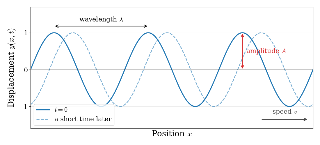
Mathematically, the displacement \(y\) of the rope at position \(x\) and time \(t\) for a wave moving to the right can be written as:

\[ y(x,t) = A\sin(kx-\omega t), \tag{1.18}\]

where we have introduced two quantities that make the formulas simpler: the wave vector, \(k=\frac{2\pi}{\lambda}\), which tells us how many radians the wave advances per unit length, and the angular frequency, \(\omega=2\pi\nu\), which tells us how many radians it advances per unit time. You can check that Eq. 1.18 repeats itself every time \(x\) increases by \(\lambda\) (at fixed \(t\)) or \(t\) increases by \(1/\nu\) (at fixed \(x\)), and that the crests move with speed \(v=\omega/k=\lambda\nu\).

A useful mathematical tool: complex waves

In quantum mechanics, waves are usually written using complex numbers instead of sines and cosines. The reason is Euler’s formula, which connects the exponential function with the trigonometric functions:

\[ e^{i\theta}=\cos\theta + i\sin\theta, \tag{1.19}\]

where \(i=\sqrt{-1}\) is the imaginary unit (complex numbers are reviewed in Sec. A.1). Using this formula, we can write a wave as:

\[ y(x,t) = A\,e^{i(kx-\omega t)} = A\cos(kx-\omega t) + iA\sin(kx-\omega t), \tag{1.20}\]

which contains both a cosine wave (the real part) and a sine wave (the imaginary part). The advantage is that exponentials are much easier to differentiate than sines and cosines: taking a derivative with respect to \(x\) simply multiplies the function by \(ik\), since \(\frac{d}{dx}e^{ikx}=ike^{ikx}\). We will start from exactly this form of a wave when we introduce the Schrödinger equation in Chapter 3.

1.3.2 The wave equation

Just as Newton’s equation describes the motion of a particle, there is an equation that describes the motion of a wave. For a wave moving along a string, it is called the classical wave equation:

\[ \frac{\partial^2 y}{\partial x^2} = \frac{1}{v^2}\frac{\partial^2 y}{\partial t^2}. \tag{1.21}\]

The left-hand side measures how curved the string is at a given point, and the right-hand side measures how fast that point accelerates up or down. In words, the equation says that the more a piece of string is curved, the faster it accelerates back towards a straight line. We can check that Eq. 1.18 is a solution: taking two derivatives with respect to \(x\) gives \(-k^2y\), and taking two derivatives with respect to \(t\) gives \(-\omega^2y\). Replacing them in Eq. 1.21, we obtain \(-k^2y=-\frac{\omega^2}{v^2}y\), which is true as long as \(v=\omega/k\), the relation between speed, frequency, and wavelength that we already found.

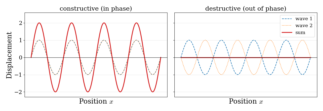
An important property of the wave equation is that it is linear: if \(y_1(x,t)\) and \(y_2(x,t)\) are two solutions, their sum, \(y_1+y_2\), is also a solution. This is called the principle of superposition, and it means that when two waves meet, their displacements simply add up. If the crests of the two waves coincide (they are in phase), they reinforce each other and produce a larger wave, which is called constructive interference. If the crests of one wave coincide with the troughs of the other (they are out of phase), they cancel each other, which is called destructive interference. The two cases are shown in Fig. 1.2. Interference is the signature of wave behavior, and we will see in Chapter 8 that it is also observed for electrons.

Figure 1.2: Superposition of two waves with the same wavelength. Left: when the waves are in phase, they add up to a wave with twice the amplitude (constructive interference). Right: when they are out of phase, they cancel each other (destructive interference).

1.3.3 Standing waves on a string

Something very interesting happens when a wave is confined, as on a guitar string of length \(L\) fixed at both ends. The waves travel along the string, bounce back at the ends, and interfere with themselves. Most of them cancel out, and only a few special patterns survive. These patterns do not travel along the string; they just oscillate up and down in place, and they are called standing waves.

To find them, we look for solutions of the wave equation in which the shape of the string does not change, but only its size, which oscillates in time:

\[ y(x,t) = \psi(x)\cos(\omega t). \tag{1.22}\]

Here \(\psi(x)\) describes the shape of the string, and \(\cos(\omega t)\) describes how it oscillates. Replacing Eq. 1.22 in the wave equation, Eq. 1.21, the time-dependent factor cancels out, and we are left with an equation for the shape only:

\[ \frac{d^2 \psi}{d x^2} = -k^2\psi(x), \qquad k=\frac{\omega}{v}. \tag{1.23}\]

The solutions of this equation are sines and cosines, \(\psi(x)=a\sin(kx)+b\cos(kx)\). Now we use the fact that the string is fixed at both ends, which gives two boundary conditions:

• At \(x=0\), the string cannot move, so \(\psi(0)=0\). Since \(\sin(0)=0\) and \(\cos(0)=1\), this requires \(b=0\), and \(\psi(x)=a\sin(kx)\).
• At \(x=L\), the string cannot move either, so \(\psi(L)=a\sin(kL)=0\). If \(a=0\) the string does not vibrate at all, so we need \(\sin(kL)=0\), which is only true when \(kL\) is a whole multiple of \(\pi\).

The second condition can only be satisfied by special values of \(k\), and therefore of the wavelength, \(\lambda=2\pi/k\), and of the frequency, \(\nu=v/\lambda\):

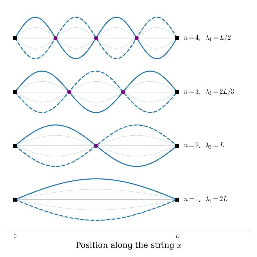
\[ k_n = \frac{n\pi}{L}, \qquad \lambda_n = \frac{2L}{n}, \qquad \nu_n = \frac{nv}{2L}, \qquad n = 1, 2, 3, \ldots \tag{1.24}\]

and the corresponding shapes are:

\[ \psi_n(x) = a\sin\left(\frac{n\pi x}{L}\right). \tag{1.25}\]

The first four standing waves are shown in Fig. 1.3.

Figure 1.3: The first four standing waves on a string of length \(L\) fixed at both ends (black squares). The solid and dashed lines show the string at its two extreme positions, and the light lines show intermediate positions. The nodes are reported as purple dots.

Three things in these results are worth noticing:

1. Quantization: a confined wave can only have certain wavelengths and frequencies, labeled by a whole number, \(n\). This is why a guitar string plays a definite note (the frequency with \(n=1\), called the fundamental) together with its overtones (\(n=2,3,\ldots\)), and not any frequency at all. Notice that nothing in the wave equation itself is quantized: the quantization comes entirely from the boundary conditions, i.e., from confining the wave.

2. Nodes: the standing wave with quantum number \(n\) has \(n-1\) points between the two ends where the string never moves, called nodes. The higher the frequency, the more nodes the wave has.

3. The link with quantum mechanics: in Chapter 4, we will solve the Schrödinger equation for an electron confined in a one-dimensional box, and we will obtain exactly the same functions as in Eq. 1.25, with the same conditions on the wavelength. The quantization of the energy of atoms and molecules has the same origin as the quantization of the notes of a guitar: a wave that is confined in a region of space.

1.3.4 Light as an electromagnetic wave

One more type of wave will be important for us: light. In the 19th century, James Clerk Maxwell showed that light is a wave of oscillating electric and magnetic fields, called an electromagnetic wave. In a vacuum, all electromagnetic waves travel at the same speed, the speed of light, \(c=2.998\times10^8\;\text{m/s}\), so Eq. 1.17 becomes:

\[ c = \lambda\nu. \tag{1.26}\]

Different wavelengths correspond to different types of radiation, which together form the electromagnetic spectrum: from radio waves (wavelengths of meters or more), to microwaves (millimeters to centimeters), infrared (micrometers), visible light (\(400\)–\(700\;\text{nm}\)), ultraviolet, X-rays, and gamma rays (shorter than a billionth of a meter). In classical physics, the energy carried by an electromagnetic wave depends on its amplitude (the brighter the light, the more energy it carries), and not on its frequency. As we will see in the next chapter, this classical picture of light is one of the first things that quantum mechanics had to change.

1.4 Chapter Review

1.4.1 Key Ideas

• Newton’s equation, \(F=m\ddot{x}\), determines the trajectory of a particle once we know the forces and the initial conditions.
• The Hamiltonian, \(H=\frac{p^2}{2m}+V(x)\), describes the same physics through the total energy, which is conserved. It is the bridge to quantum mechanics.
• Charged particles interact through the Coulomb potential energy, \(V(r)=\frac{q_1q_2}{4\pi\varepsilon_0 r}\), which is negative (attractive) for an electron and a nucleus.
• Waves are described by their wavelength, frequency, and speed, \(v=\lambda\nu\), and they are conveniently written as complex exponentials using Euler’s formula.
• A wave confined between two fixed points can only have certain wavelengths: confinement leads to quantization, and higher frequencies mean more nodes.

1.4.2 Study Questions

1. If we know the net force acting on a particle, and its position and velocity at one instant, Newton’s equation allows us to:

1. calculate only its average position
2. calculate only the probability of finding it at each position
3. calculate its position at any future (or past) time
4. calculate its energy, but not its position
5. calculate its position only if no force acts on it

---

2. The momentum of a particle of mass \(m\) moving with velocity \(\dot{x}\) is:

1. \(p=\frac{1}{2}m\dot{x}^2\)
2. \(p=m\ddot{x}\)
3. \(p=\dot{x}/m\)
4. \(p=mgx\)
5. \(p=m\dot{x}\)

---

3. Which of the following is the Hamiltonian of a particle of mass \(m\) moving in one dimension with potential energy \(V(x)\)?

1. \(H=\frac{p^2}{2m}-V(x)\)
2. \(H=m\ddot{x}\)
3. \(H=\frac{1}{2}mp^2+V(x)\)
4. \(H=\frac{p^2}{2m}+V(x)\)
5. \(H=p\,V(x)\)

---

4. Why is the Hamiltonian, rather than Newton’s equation, the starting point of quantum mechanics?

1. because it is easier to integrate than Newton’s equation
2. because it describes the system through its energy, which keeps its meaning even when trajectories do not
3. because it does not depend on the potential energy
4. because it gives different results from Newton’s equation for heavy particles
5. because forces do not exist in quantum mechanics

---

5. The Coulomb force between an electron and a proton is:

1. repulsive, because the two charges have opposite signs
2. zero, because the two charges cancel each other
3. attractive, because the two charges have opposite signs
4. attractive only at large distances
5. independent of the distance between the particles

---

6. The electrostatic potential energy \(V\) of two point charges \(q_1\) and \(q_2\) separated by a distance \(r\) is:

1. \(V = \dfrac{1}{4\pi \varepsilon_0} \dfrac{q_1 q_2}{r^2}\)
2. \(V = \dfrac{1}{4\pi \varepsilon_0} q_1 q_2 r\)
3. \(V = q_1 q_2 r^2\)
4. \(V = \dfrac{1}{4\pi \varepsilon_0} \dfrac{q_1 q_2}{r}\)
5. \(V = \dfrac{q_1 + q_2}{r}\)

---

7. The speed \(v\), wavelength \(\lambda\), and frequency \(\nu\) of a wave are related by:

1. \(v=\lambda/\nu\)
2. \(v=\nu/\lambda\)
3. \(v=2\pi\lambda\nu\)
4. \(v=\lambda^2\nu\)
5. \(v=\lambda\nu\)

---

8. Euler’s formula, which allows us to write waves using complex exponentials, is:

1. \(e^{i\theta}=\cos\theta+i\sin\theta\)
2. \(e^{i\theta}=\cos\theta-i\sin\theta\)
3. \(e^{i\theta}=\sin\theta+i\cos\theta\)
4. \(e^{\theta}=\cos\theta+\sin\theta\)
5. \(e^{i\theta}=i\cos\theta\sin\theta\)

---

9. A guitar string of length \(L\) is fixed at both ends. Which wavelengths can its standing waves have?

1. any wavelength
2. only \(\lambda_n=2L/n\), with \(n=1,2,3,\ldots\)
3. only \(\lambda=L\)
4. only wavelengths longer than \(2L\)
5. only \(\lambda_n=nL\), with \(n=1,2,3,\ldots\)

---

10. How many nodes (points that never move, not counting the two fixed ends) does the standing wave with quantum number \(n\) have?

1. \(n-1\)
2. \(n\)
3. \(n+1\)
4. \(2n\)
5. none

---

ExampleAnswers

1.c, 2.e, 3.d, 4.b, 5.c, 6.d, 7.e, 8.a, 9.b, 10.a

---

1. Notice that \(\mathbf{r}\) \(\in\) \(\mathbb{R}^{3}\) is the position vector and \(\dot{\mathbf{r}}\) \(\in\) \(\mathbb{R}^{3}\) is the velocity vector. As such, all the equations of classical mechanics are vector equations in 3-dimensional space, and not just simple numerical equations. To simplify the picture, we can restrict ourselves to a 1-dimensional space, replace \(\mathbf{r}\) with \(x\), and forget the complications of vector algebra, as we do in the examples.

2. This example is based on Rhett Allain’s blog post on classical mechanics.

3. Can you write a python program to do this calculation?

4. The Lagrangian formulation is very powerful for complicated mechanical systems, such as a pendulum hanging from a moving support, but we will not need it in this textbook. Interested readers can find an introduction in the Wikipedia article on Lagrangian mechanics.