9 Gibbs Free Energy

In this chapter, we will concentrate on chemical processes that happen at constant \(T\) and constant \(P\).³⁴ As such, we will focus our attention on the Gibbs free energy.

9.1 Gibbs Equation

Recalling from chapter 8, the definition of \(G\) is:

\[\begin{equation} G = U -TS +PV = H-TS, \tag{9.1} \end{equation}\]

which, taking the differential at constant \(T\) and \(P\), becomes:

\[\begin{equation} dG = dH \; \overbrace{-SdT}^{=0} -TdS = dH -TdS. \tag{9.2} \end{equation}\]

Integrating eq. (9.2) between the initial and final states of a process results in:

\[\begin{equation} \begin{aligned} \int_i^f dG &= \int_i^f dH -T \int_i^f dS \\ \\ \Delta G &= \Delta H -T \Delta S \end{aligned} \tag{9.3} \end{equation}\]

which is the famous Gibbs equation for \(\Delta G\). Using Definition 8.2, we can use \(\Delta G\) to infer the spontaneity of a chemical process that happens at constant \(T\) and \(P\) using \(\Delta G \leq 0\). If we set ourselves at standard conditions, we can calculate the standard Gibbs free energy of formation, \(\Delta_{\text{rxn}} G^{-\kern-6pt{\ominus}\kern-6pt-}\), for any reaction as:

\[\begin{equation} \begin{aligned} \Delta_{\text{rxn}} G^{-\kern-6pt{\ominus}\kern-6pt-}&= \Delta_{\text{rxn}} H^{-\kern-6pt{\ominus}\kern-6pt-}-T \Delta_{\text{rxn}} S^{-\kern-6pt{\ominus}\kern-6pt-}\\ \\ &= \sum_i \nu_i \Delta_{\mathrm{f}} H_i^{-\kern-6pt{\ominus}\kern-6pt-}- T \sum_i \nu_i S_i^{-\kern-6pt{\ominus}\kern-6pt-}, \end{aligned} \tag{9.4} \end{equation}\]

where \(\Delta_{\mathrm{f}} H_i^{-\kern-6pt{\ominus}\kern-6pt-}\) are the standard enthalpies of formation, \(S_i^{-\kern-6pt{\ominus}\kern-6pt-}\) are the standard entropies, and \(\nu_i\) are the stoichiometric coefficients for every species \(i\) involved in the reaction. All these quantities are commonly available, and we have already discussed their usage in chapters 4 and 7, respectively.³⁵

The following four options are possible for \(\Delta G^{-\kern-6pt{\ominus}\kern-6pt-}\) of a chemical reaction:

\(\Delta G^{-\kern-6pt{\ominus}\kern-6pt-}\)		\(\Delta H^{-\kern-6pt{\ominus}\kern-6pt-}\)	\(\Delta S^{-\kern-6pt{\ominus}\kern-6pt-}\)	Spontaneous?
–	if	–	+	Always
+	if	+	–	Never
–/+	if	–	–	Depends on \(T\): \(\scriptstyle{\text{spontaneous at low } T}\)
+/–	if	+	+	Depends on \(T\): \(\scriptstyle{\text{spontaneous at high } T}\)

Or, in other words:

• Exothermic reactions that increase the entropy are always spontaneous.
• Endothermic reactions that reduce the entropy are always non-spontaneous.
• For the other two cases, the spontaneity of the reaction depends on the temperature:
  • Exothermic reactions that reduce the entropy are spontaneous at low \(T\).
  • Endothermic reactions that increase the entropy are spontaneous at high \(T\).

A simple criterion to evaluate the entropic contribution of a reaction is to look at the total number of moles of the reactants and the products (as the sum of the stoichiometric coefficients). If the reaction is producing more molecules than it destroys \(\left( \left| \sum_\text{products} \nu_i \right| > \left| \sum_\text{reactants} \nu_i \right| \right)\), it will increase the entropy. Vice versa, if the total number of moles in a reaction is reducing \(\left( \left| \sum_\text{products} \nu_i \right| < \left| \sum_\text{reactants} \nu_i \right| \right)\), the entropy will also reduce.

As we saw in section 8.2, the natural variables of the Gibbs free energy are the temperature, \(T\), the pressure, \(P\), and chemical composition, as the number of moles \(\{n_i\}\). The Gibbs free energy can therefore be expressed using the total differential as (see also, last formula in eq. (8.16)):

\[\begin{equation} dG(T,P,\{n_i\}) = \mkern-18mu \underbrace{\left(\frac{\partial G}{\partial T} \right)_{P,\{n_i\}}}_{\text{temperature dependence}} \mkern-36mu dT + \underbrace{\left(\frac{\partial G}{\partial P} \right)_{T,\{n_i\}}}_{\text{pressure dependence}} \mkern-36mu dP + \sum_i \underbrace{\left(\frac{\partial G}{\partial n_i} \right)_{T,P,\{n_{j \neq i}\}}}_{\text{composition dependence}} \mkern-36mu dn_i. \tag{9.5} \end{equation}\]

If we know the behavior of \(G\) as we vary each of the three natural variables independently of the other two, we can reconstruct the total differential \(dG\). Each of these terms represents a coefficient in eq. (9.5), which are given in eq. (8.17).

9.2 Temperature Dependence of \(\Delta G\)

\[ \left(\frac{\partial G}{\partial T} \right)_{P,\{n_i\}}=-S \]

Let’s analyze the first coefficient that gives the dependence of the Gibbs energy on temperature. Since this coefficient is equal to \(-S\) and the entropy is always positive, \(G\) must decrease when \(T\) increases at constant \(P\) and \(\{n_i\}\), and vice versa.

If we replace this coefficient for \(-S\) in the Gibbs equation, eq. (9.3), we obtain:

\[\begin{equation} \Delta G = \Delta H + T \left(\frac{\partial \Delta G}{\partial T} \right)_{P,\{n_i\}}, \tag{9.6} \end{equation}\]

and since eq. (9.6) includes both \(\Delta G\) and its partial derivative with respect to temperature \(\left(\frac{\partial \Delta G}{\partial T} \right)_{P,\{n_i\}}\) we need to rearrange it to include the temperature derivative only. To do so, we can start by evaluating the partial derivative of \(\left( \frac{\Delta G}{T} \right)\) using the chain rule:

\[\begin{equation} \left[ \frac{\partial\left( \frac{\Delta G}{T} \right)}{\partial T} \right]_{P,\{n_i\}} = \frac{1}{T} \left(\frac{\partial \Delta G}{\partial T} \right)_{P,\{n_i\}} - \frac{1}{T^2}\Delta G, \tag{9.7} \end{equation}\]

which, replacing \(\Delta G\) from eq. (9.6) into eq. (9.7), becomes:

\[\begin{equation} \begin{aligned} \left[ \frac{\partial\left( \frac{\Delta G}{T} \right)}{\partial T} \right]_{P,\{n_i\}} &= \frac{1}{T} \left(\frac{\partial \Delta G}{\partial T} \right)_{P,\{n_i\}} - \frac{1}{T^2} \left[ \Delta H + T \left(\frac{\partial \Delta G}{\partial T} \right)_{P,\{n_i\}} \right] \\ &= \frac{1}{T} \left(\frac{\partial \Delta G}{\partial T} \right)_{P,\{n_i\}}- \frac{\Delta H}{T^2}-\frac{1}{T} \left(\frac{\partial \Delta G}{\partial T} \right)_{P,\{n_i\}}, \end{aligned} \tag{9.8} \end{equation}\]

which simplifies to:

\[\begin{equation} \begin{aligned} \left[ \frac{\partial\left( \frac{\Delta G}{T} \right)}{\partial T} \right]_{P,\{n_i\}} &= - \frac{\Delta H}{T^2}. \end{aligned} \tag{9.9} \end{equation}\]

Equation (9.9) is known as the Gibbs–Helmholtz equation, and is useful in its integrated form to calculate the Gibbs free energy for a chemical reaction at any temperature \(T\) by knowing just the standard Gibbs free energy of formation and the standard enthalpy of formation for the individual species, which are usually reported at \(T=298\;\text{K}\). The integration is performed as follows:

\[\begin{equation} \begin{aligned} \int_{T_i=298 \;\text{K}}^{T_f=T} \frac{\partial\left( \frac{\Delta_{\text{rxn}} G}{T} \right)}{\partial T} &= - \int_{T_i=298 \;\text{K}}^{T_f=T} \frac{\Delta_{\text{rxn}} H}{T^2} \\ \\ \frac{\Delta_{\text{rxn}} G^{-\kern-6pt{\ominus}\kern-6pt-}(T)}{T} &= \frac{\Delta_{\text{rxn}} G^{-\kern-6pt{\ominus}\kern-6pt-}}{298 \;\text{K}} + \Delta_{\text{rxn}} H^{-\kern-6pt{\ominus}\kern-6pt-}\left( \frac{1}{T} -\frac{1}{298 \;\text{K}} \right), \end{aligned} \tag{9.10} \end{equation}\]

giving the integrated Gibbs–Helmholtz equation:

\[\begin{equation} \frac{\Delta_{\text{rxn}} G^{-\kern-6pt{\ominus}\kern-6pt-}(T)}{T} = \frac{\sum_i \nu_i \Delta_{\text{f}} G_i^{-\kern-6pt{\ominus}\kern-6pt-}}{298 \;\text{K}} + \sum_i \nu_i \Delta_{\text{f}} H_i^{-\kern-6pt{\ominus}\kern-6pt-}\left( \frac{1}{T} -\frac{1}{298 \;\text{K}} \right) \tag{9.11} \end{equation}\]

9.3 Pressure Dependence of \(\Delta G\)

\[ \left(\frac{\partial G}{\partial P} \right)_{T,\{n_i\}}=V \]

We can now turn the attention to the second coefficient that gives how the Gibbs free energy changes when the pressure change. To do this, we put the system at constant \(T\) and \(\{n_i\}\), and then we consider infinitesimal variations of \(G\). From eq. (8.8):

\[\begin{equation} dG = VdP -SdT +\sum_i\mu_i dn_i \quad \xrightarrow{\text{constant}\; T,\{n_i\}} \quad dG = VdP, \tag{9.12} \end{equation}\]

which is the differential equation that we were looking for. To study changes of \(G\) for macroscopic changes in \(P\), we can integrate eq. (9.12) between initial and final pressures, and considering an ideal gas, we obtain:

\[\begin{equation} \begin{aligned} \int_i^f dG &= \int_i^f VdP \\ \Delta G &= nRT \int_i^f \frac{dP}{P} = nRT \ln \frac{P_f}{P_i}. \end{aligned} \tag{9.13} \end{equation}\]

If we take \(P_i = P^{-\kern-6pt{\ominus}\kern-6pt-}= 1 \, \text{bar}\), we can rewrite eq. (9.13) as:

\[\begin{equation} G = G^{-\kern-6pt{\ominus}\kern-6pt-}+ nRT \ln \frac{P_f}{P^{-\kern-6pt{\ominus}\kern-6pt-}}, \tag{9.14} \end{equation}\]

which is useful to convert standard Gibbs free energies of formation at pressures different than standard pressure, using:

\[\begin{equation} \Delta_{\text{f}} G = \Delta_{\text{f}} G^{-\kern-6pt{\ominus}\kern-6pt-}+ nRT \ln \frac{P_f}{\underbrace{P^{-\kern-6pt{\ominus}\kern-6pt-}}_{=1 \; \text{bar}}} = \Delta_{\text{f}} G^{-\kern-6pt{\ominus}\kern-6pt-}+ nRT \ln P_f \tag{9.15} \end{equation}\]

For liquids and solids, \(V\) is essentially independent of \(P\) (liquids and solids are incompressible), and eq. (9.12) can be integrated as:

\[\begin{equation} \Delta G = \int_i^f VdP = V \int_i^f dP = V \Delta P. \tag{9.16} \end{equation}\]

The plots in Figure 9.1 show the remarkable difference in the behaviors of \(\Delta_{\text{f}} G\) for a gas and for a liquid, as obtained from eqs. (9.13) and (9.16).

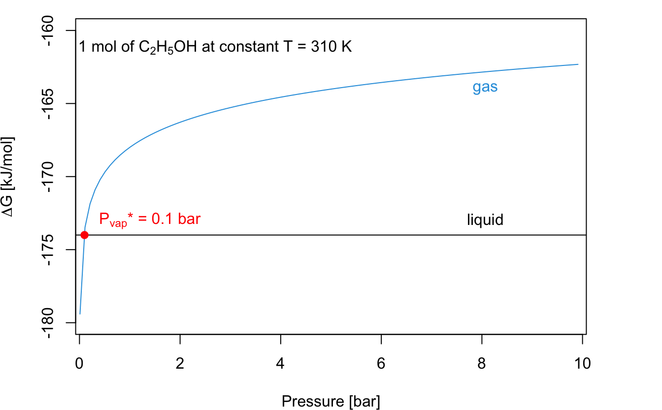
Figure 9.1: Dependence of the Gibbs Free Energy of Formation of Liquid and Gaseous Ethanol at T = 310 K. The Curves Cross at the Vapor Pressure of Liquid Ethanol at this Temperature, which is 0.1 bar.

9.4 Composition Dependence of \(\Delta G\)

\[ \left(\frac{\partial G}{\partial n_i} \right)_{T,P}=\mu_i \]

The third and final coefficient gives the chemical potential as the dependence of \(G\) on the chemical composition at constant \(T\) and \(P\). Similarly to the previous cases, we can take the definition of the coefficient and integrate it directly between the initial and final stages of a reaction. If we consider a reaction product, pure substance \(i\), at the beginning of the reaction there will be no moles of it \(n_i=0\), and consequently \(G=0\).³⁶ We can then integrate the left-hand side between zero and the number of moles of product at the end of the reaction, \(n\), and the right-hand side between zero and the Gibbs free energy of the product, \(G\). The integral will become:

\[\begin{equation} \int_0^G d G = \int_0^n \mu^* dn, \tag{9.17} \end{equation}\]

where \(\mu^*\) indicates the chemical potential of a pure substance, which is independent on the number of moles by definition. As such, eq. (9.17) becomes:

\[\begin{equation} \int_0^G d G = \mu^* \int_0^n dn \quad \rightarrow \quad G = \mu^* n \quad \rightarrow \quad \mu^* = \frac{G}{n}, \tag{9.18} \end{equation}\]

which gives a straightforward interpretation of the chemical potential of a pure substance as the molar Gibbs free energy.

We can start from eq. (9.14) and write for a pure substance that is brought from \(P_i=P^{-\kern-6pt{\ominus}\kern-6pt-}\) to \(P_f=P\) at constant \(T\):

\[\begin{equation} G - G^{-\kern-6pt{\ominus}\kern-6pt-}= nRT \ln \frac{P}{P^{-\kern-6pt{\ominus}\kern-6pt-}}, \tag{9.19} \end{equation}\]

dividing both sides by \(n\), we obtain:

\[\begin{equation} \frac{G}{n} - \frac{G^{-\kern-6pt{\ominus}\kern-6pt-}}{n} = RT \ln \frac{P}{P^{-\kern-6pt{\ominus}\kern-6pt-}}, \tag{9.20} \end{equation}\]

which, for a pure substance at \(P^{-\kern-6pt{\ominus}\kern-6pt-}= 1 \;\text{bar}\), becomes:

\[\begin{equation} \mu^* - \mu^{-\kern-6pt{\ominus}\kern-6pt-}= RT \ln P. \tag{9.21} \end{equation}\]

Notice that, while we use the pressure of the gas inside the logarithm in eq. (9.21), the quantity is formally divided by the standard pressure \(P^{-\kern-6pt{\ominus}\kern-6pt-}= 1 \;\text{bar}\), and therefore it is a dimensionless quantity, as it should be. For simplicity of notation, however, we will omit the division by \(P^{-\kern-6pt{\ominus}\kern-6pt-}\) in the remaining of this textbook, especially wherever it does not create confusion. Let’s now consider a mixture of ideal gases, and let’s try to find out whether the chemical potential of a pure gas inside the mixture, \(\mu_i^{\text{mixture}}\), is the same as its chemical potential outside the mixture, \(\mu^*\). To do so, we can use eq. (9.21) and replace the pressure \(P\) with the partial pressure \(P_i\):

\[\begin{equation} \mu_i^{\text{mixture}} = \mu_i^{-\kern-6pt{\ominus}\kern-6pt-}+ RT \ln P_i, \tag{9.22} \end{equation}\]

where the partial pressure \(P_i\) can be obtained from the simple relation that is known as Dalton’s Law:

\[\begin{equation} P_i = y_i P, \tag{9.23} \end{equation}\]

with \(y_i\) being the concentration of gas \(i\) measured as a mole fraction in the gas phase \(y_i=\frac{n_i}{n_{\text{TOT}}} < 1\). Replacing eq. (9.23) into eq. (9.22), we obtain:

\[\begin{equation} \begin{aligned} \mu_i^{\text{mixture}} &= \mu_i^{-\kern-6pt{\ominus}\kern-6pt-}+ RT \ln (y_i P) \\ &= \underbrace{\mu_i^{-\kern-6pt{\ominus}\kern-6pt-}+ RT \ln P}_{\mu_i^*} + RT \ln y_i, \end{aligned} \tag{9.24} \end{equation}\]

which then reduces to the following equation:

\[\begin{equation} \mu_i^{\text{mixture}} = \mu_i^* + RT \ln y_i. \tag{9.25} \end{equation}\]

Analyzing eq. (9.25), we can immediately see that, since \(y_i < 1\):

\[\begin{equation} \mu_i^{\text{mixture}} < \mu_i^*, \tag{9.26} \end{equation}\]

or, in other words, the chemical potential of a substance in the mixture is always lower than the chemical potential of the pure substance. If we consider a process where we start from two separate pure ideal gases and finish with a mixture of the two, we can calculate the change in Gibbs free energy due to the mixing process with:

\[\begin{equation} \Delta_{\text{mixing}} G = \sum n_i \left( \mu_i^{\text{mixture}} - \mu_i^* \right) < 0, \tag{9.27} \end{equation}\]

or, in other words, the process is spontaneous under all circumstances, and pure ideal gases will always mix.

---

34. The majority of chemical reactions in a lab happens at those conditions, and all biological functions happen at those conditions as well.↩︎

35. It is not uncommon to see values of \(\Delta_{\text{f}} G^{-\kern-6pt{\ominus}\kern-6pt-}\) tabulated alongside \(\Delta_{\mathrm{f}} H^{-\kern-6pt{\ominus}\kern-6pt-}\) and \(S_i^{-\kern-6pt{\ominus}\kern-6pt-}\), which simplifies even further the calculation. In fact, a comprehensive list of standard Gibbs free energy of formation of inorganic and organic compounds is reported in the appendix of this book 15. For cases where \(\Delta_{\text{f}} G^{-\kern-6pt{\ominus}\kern-6pt-}\) are not reported, they can always be calculated by their constituents.↩︎

36. For reactants, the same situation usually applies but in reverse. More complicated cases where the reaction does not consume all reactants are possible, but insignificant for the following treatment.↩︎