10 Chemical Equilibrium
10.1 Reaction Quotient and Equilibrium Constant
Let’s consider a prototypical reaction at constant \(T,P\):
\[\begin{equation} a\mathrm{A} + b\mathrm{B} \rightarrow c\mathrm{C} + d\mathrm{D} \tag{10.1} \end{equation}\]
The Gibbs energy of the reaction is defined as:
\[\begin{equation} \Delta_{\text{rxn}} G = G_{\text{products}} - G_{\text{reactants}} = G^{\text{C}} + G^{\text{D}} - G^{\text{A}}-G^{\text{B}}, \tag{10.2} \end{equation}\]
and replacing the absolute Gibbs energies with the chemical potentials \(\mu_i\), we obtain:
\[\begin{equation} \Delta_{\text{rxn}} G = c \mu_{\text{C}} + d \mu_{\text{D}} - a \mu_{\text{A}}- b\mu_{\text{B}}. \tag{10.3} \end{equation}\]
Assuming the reaction is happening in the gas phase, we can then use eq. (9.22) to replace the chemical potentials with their value in the reaction mixture, as:
\[\begin{equation} \begin{aligned} \mkern-60mu \Delta_{\text{rxn}} G =& \; c (\mu_{\text{C}}^{-\kern-6pt{\ominus}\kern-6pt-}+RT \ln P_{\text{C}}) + d (\mu_{\text{D}}^{-\kern-6pt{\ominus}\kern-6pt-}+RT \ln P_{\text{D}}) +\\ & - a (\mu_{\text{A}}^{-\kern-6pt{\ominus}\kern-6pt-}+RT \ln P_{\text{A}}) - b (\mu_{\text{B}}^{-\kern-6pt{\ominus}\kern-6pt-}+RT \ln P_{\text{B}}) \\ =& \; \underbrace{c \mu_{\text{C}}^{-\kern-6pt{\ominus}\kern-6pt-}+ d \mu_{\text{D}}^{-\kern-6pt{\ominus}\kern-6pt-}- a \mu_{\text{A}}^{-\kern-6pt{\ominus}\kern-6pt-}- b\mu_{\text{B}}^{-\kern-6pt{\ominus}\kern-6pt-}}_{\Delta_{\text{rxn}} G^{-\kern-6pt{\ominus}\kern-6pt-}} +RT \ln \frac{P_{\text{C}}^c \cdot P_{\text{D}}^d}{P_{\text{A}}^a \cdot P_{\text{B}}^b}. \end{aligned} \tag{10.4} \end{equation}\]
We can define a new quantity called the reaction quotient as a function of the partial pressures of each substance:44
\[\begin{equation} Q_P = \frac{P_{\text{C}}^c \cdot P_{\text{D}}^d}{P_{\text{A}}^a \cdot P_{\text{B}}^b}, \tag{10.5} \end{equation}\]
and we can then simply rewrite eq. (10.4) using eq. (10.5) as:
\[\begin{equation} \Delta_{\text{rxn}} G = \Delta_{\text{rxn}} G^{-\kern-6pt{\ominus}\kern-6pt-}+ RT \ln Q_P. \tag{10.6} \end{equation}\]
This equation tells us that the sign of \(\Delta_{\text{rxn}} G\) is influenced by the reaction quotient \(Q_P\). For a spontaneous reaction at the beginning, the partial pressures of the reactants are much higher than the partial pressures of the products, therefore \(Q_P \ll 1\) and \(\Delta_{\text{rxn}} G < 0\), as we expect. As the reaction proceeds, the partial pressures of the products will increase, while the partial pressures of the reactants will decrease. Consequently, both \(Q_P\) and \(\Delta_{\text{rxn}} G\) will increase. The reaction will completely stop when \(\Delta_{\text{rxn}} G = 0\), which is the chemical equilibrium point. At the reaction equilibrium:
\[\begin{equation} \Delta_{\text{rxn}} G = 0 = \Delta_{\text{rxn}} G^{-\kern-6pt{\ominus}\kern-6pt-}+ RT \ln K_P, \tag{10.7} \end{equation}\]
where we have defined a new quantity called equilibrium constant, as the value the reaction quotient assumes when the reaction reaches equilibrium, and we have denoted it with the symbol \(K_P\).45 From eq. (10.7) we can derive the following fundamental equation on the standard Gibbs energy of reaction:
\[\begin{equation} \Delta_{\text{rxn}} G^{-\kern-6pt{\ominus}\kern-6pt-}= - RT \ln K_P. \tag{10.8} \end{equation}\]
To extend the concept of \(K_P\) beyond the four species in the prototypical reaction (10.1), we can use the product of a series symbol \(\left( \prod_i \right)\), and write:
\[\begin{equation} K_P=\prod_i P_{i,\text{eq}}^{\nu_i}, \tag{10.9} \end{equation}\]
where \(P_{i,\text{eq}}\) are the partial pressure of each species at equilibrium. Eq. (10.9) is in principle valid for ideal gases only. However, reaction involving ideal gases are pretty rare. As such, we can further extend the concept of equilibrium constant and write:
\[\begin{equation} K_{\text{eq}} =\prod_i a_{i,\text{eq}}^{\nu_i}, \tag{10.10} \end{equation}\]
where we have replaced the partial pressure at equilibrium, \(P_{i,\text{eq}}\), with a new concept introduced initially by Gilbert Newton Lewis (1875–1946),46 that he termed activity, and represented by the letter \(a\). For ideal gases, it is clear that \(a_i=P_i/P^{-\kern-6pt{\ominus}\kern-6pt-}\). For non-ideal gases, the activity is equal to the fugacity \(a_i=f_i/P^{-\kern-6pt{\ominus}\kern-6pt-}\), a concept that we will investigate in the next chapter. For pure liquids and solids, the activity is simply \(a_i=1\). For diluted solutions, the activity is equal to a measured concentration (such as, for example, the mole fraction \(x_i\) in the liquid phase, and \(y_i\) in the gas phase, or the molar concentration \([i]/[i]^{-\kern-6pt{\ominus}\kern-6pt-}\) with \([i]^{-\kern-6pt{\ominus}\kern-6pt-}= 1\;\text[mol/L]\)). Finally for concentrated solutions, the activity is related to the measured concentration via an activity coefficient. We will return to the concept of activity in chapter 13, when we will specifically deal with solutions. For now, it is interesting to use the activity to write the definition of the following two constants:
\[\begin{equation} K_y =\prod_i \left( y_{i,\text{eq}} \right)^{\nu_i} \qquad \qquad \qquad \qquad K_C =\left( \prod_i [i]_{\text{eq}}/[i]^{-\kern-6pt{\ominus}\kern-6pt-}\right)^{\nu_i}, \tag{10.11} \end{equation}\]
which can then be related with \(K_P\) for a mixture of ideal gases using:
\[\begin{equation} P_i = y_i P \qquad \qquad \qquad P_i=\frac{n_i}{V}RT=[i]RT, \tag{10.12} \end{equation}\]
which then results in:
\[\begin{equation} K_P = K_y\cdot \left(\frac{P}{P^{-\kern-6pt{\ominus}\kern-6pt-}}\right)^{\Delta \nu} \qquad \qquad K_P = K_C \left( \frac{[i]^{-\kern-6pt{\ominus}\kern-6pt-}RT}{P^{-\kern-6pt{\ominus}\kern-6pt-}} \right)^{\Delta \nu}, \tag{10.13} \end{equation}\]
with \(\Delta \nu =\sum_i \nu_i\).
Using the general equilibrium constant, \(K_{\text{eq}}\), we can also rewrite the fundamental equation on \(\Delta_{\text{rxn}} G^{-\kern-6pt{\ominus}\kern-6pt-}\) that we derived in eq. (10.8) to be applicable at most conditions, as:
\[\begin{equation} \Delta_{\text{rxn}} G^{-\kern-6pt{\ominus}\kern-6pt-}= - RT \ln K_{\text{eq}}, \tag{10.14} \end{equation}\]
and since \(\Delta_{\text{rxn}} G^{-\kern-6pt{\ominus}\kern-6pt-}\) depends on \(T,P\) and \(\{n_i\}\), it is useful to explore how \(K_{\text{eq}}\) depends on those variables as well.
10.2 Temperature Dependence of \(K_{\text{eq}}\)
To study the temperature dependence of \(K_{\text{eq}}\) we can use eq. (10.14) for the general equilibrium constant and write:
\[\begin{equation} \ln K_{\text{eq}} = -\frac{\Delta G^{-\kern-6pt{\ominus}\kern-6pt-}}{RT}, \tag{10.15} \end{equation}\]
which we can then differentiate with respect to temperature at constant \(P,\{n_i\}\) on both sides:
\[\begin{equation} \left( \frac{\partial \ln K_{\text{eq}}}{\partial T} \right)_{P,\{n_i\}} = -\frac{1}{R} \left[ \frac{\partial \left( \frac{\Delta G^{-\kern-6pt{\ominus}\kern-6pt-}}{T} \right)}{\partial T} \right]_{P,\{n_i\}}, \tag{10.16} \end{equation}\]
and, using Gibbs-Helmholtz equation (eq. (9.9)) to simplify the left hand side, becomes:
\[\begin{equation} \left( \frac{\partial \ln K_{\text{eq}}}{\partial T} \right)_{P,\{n_i\}} = -\frac{1}{R} \left( -\frac{\Delta H^{-\kern-6pt{\ominus}\kern-6pt-}}{T^2} \right) = \frac{\Delta H^{-\kern-6pt{\ominus}\kern-6pt-}}{RT^2}, \tag{10.17} \end{equation}\]
which gives the dependence of \(\ln K_{\text{eq}}\) on \(T\) that we were looking for. Eq. (10.17) is also called van ’t Hoff equation,47 and it is the mathematical expression of Le Chatelier’s principle. The simplest interpretation is as follows:
- For an exothermic reaction (\(\Delta H^{-\kern-6pt{\ominus}\kern-6pt-}< 0\)): \(K_{\text{eq}}\) will decrease as the temperature increases.
- For an endothermic reaction (\(\Delta H^{-\kern-6pt{\ominus}\kern-6pt-}> 0\)): \(K_{\text{eq}}\) will increase as the temperature increases.
If we integrate the van ’t Hoff equation between two arbitrary points at constant \(P\), and assuming constant \(\Delta H^{-\kern-6pt{\ominus}\kern-6pt-}\), we obtain the following:
\[\begin{equation} \int_1^2 d \ln K_{\text{eq}} = \frac{\Delta H^{-\kern-6pt{\ominus}\kern-6pt-}}{R} \int_1^2 \frac{dT}{T^2}, \tag{10.18} \end{equation}\]
which leads to the linear equation:
\[\begin{equation} \ln K_{\text{eq}}(2) = \ln K_{\text{eq}}(1) - \frac{\Delta H^{-\kern-6pt{\ominus}\kern-6pt-}}{R} \left( \frac{1}{T_2}-\frac{1}{T_1} \right). \tag{10.19} \end{equation}\]
which is the equation that produces the so-called van ’t Hoff plots, from which \(\Delta H^{-\kern-6pt{\ominus}\kern-6pt-}\) can be experimentally determined:
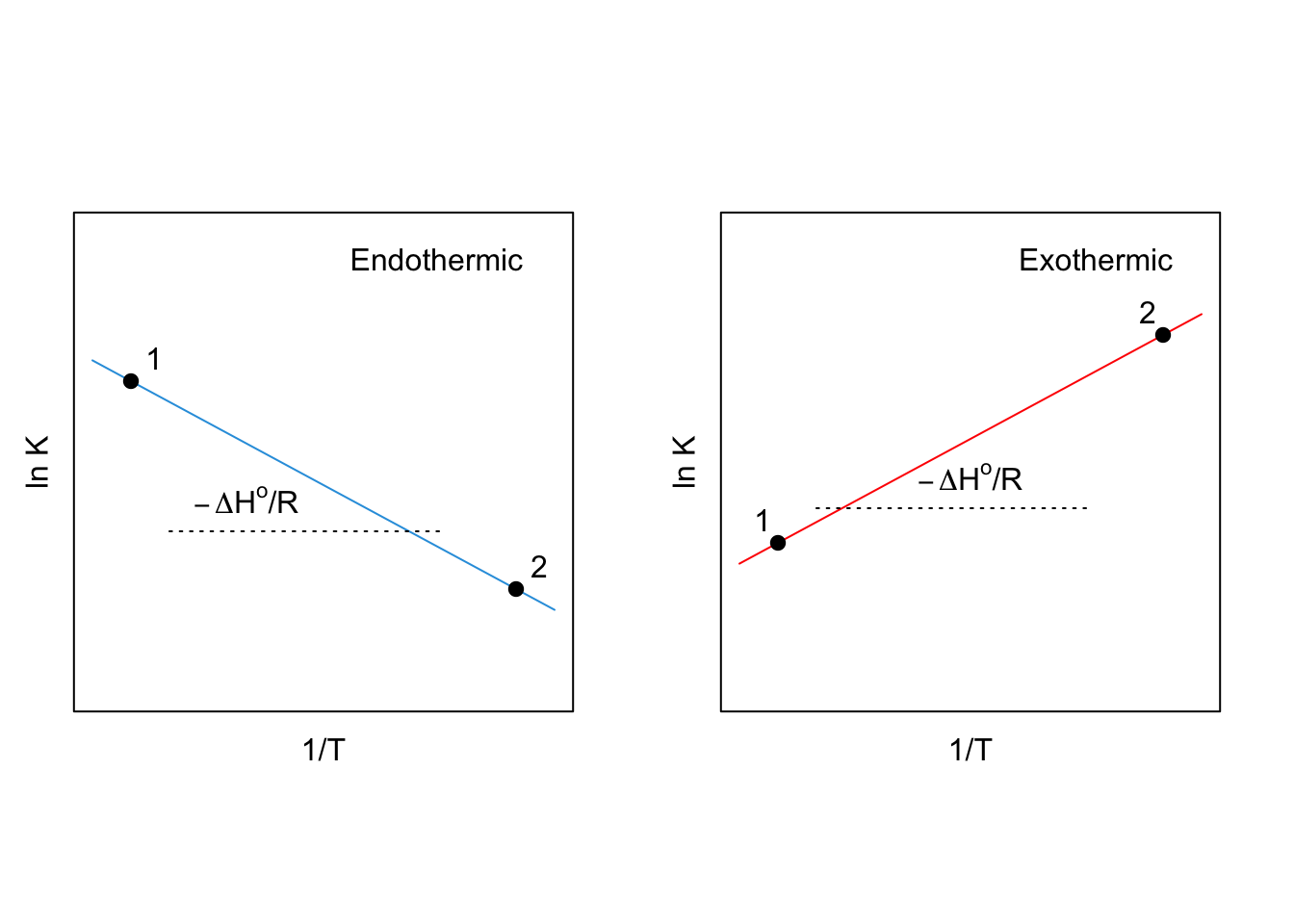
Figure 10.1: Van ’t Hoff Plots for an Endothermic (Left, Blue) and an Exothermic (Right, Red) Reactions at Constant P.
10.3 Pressure and Composition Dependence of \(K_{\text{eq}}\)
While \(K_P\) is independent of both total pressure and number of moles for an ideal gas, the same is not necessarily true for the other equilibrium constants.
\[\begin{equation} \left( \frac{\partial K_P}{\partial P} \right)_{T,\{n_i\}} = 0 \qquad \qquad \left( \frac{\partial K_P}{\partial n_i} \right)_{T,P} =0. \tag{10.20} \end{equation}\]
For example, it is easy to look at eq. (10.13) and determine that \(K_y\) usually depends on \(P\).48 Using Dalton’s Law, eq. (9.23), we can also notice that the equilibrium partial pressures of the reactants and products in a gas-phase reaction can be expressed in terms of their equilibrium mole fractions \(y_i\) and the total pressure \(P\). As such, we can use \(K_y\) to demonstrate that the equilibrium mole fractions will change when \(P\) changes,49 as it is demonstrated by the following exercise.
Exercise 10.1 Calculate the mole fraction change for the dissociation of \(\mathrm{Cl}_{2(g)}\) when the pressure is increased from \(P^{-\kern-6pt{\ominus}\kern-6pt-}\) to \(P_f=2.5 \;\text{bar}\) at constant \(T=2\,298\;\mathrm{K}\), knowing that \(\Delta_{\mathrm{f}} G^{-\kern-6pt{\ominus}\kern-6pt-}_{\mathrm{Cl}_{(g)}} = 105.3 \;\text{kJ/mol}\) and \(\Delta_{\mathrm{f}} H^{-\kern-6pt{\ominus}\kern-6pt-}_{\mathrm{Cl}_{(g)}} = 121.3 \;\text{kJ/mol}\), and remembering that both of these values are tabulated at \(T=298\;\text{K}\).
Solution: Let’s consider the reaction: \[ \mathrm{Cl}_{2(g)} \rightleftarrows 2 \mathrm{Cl}_{(g)} \]
We can divide the exercise into two parts. In the first one, we will deal with calculating the equilibrium constant at \(T=2\,298\;\mathrm{K}\) from the data at \(T=298\;\mathrm{K}\). In the second one, we will calculate the change in mole fraction when the pressure is increased from \(P^{-\kern-6pt{\ominus}\kern-6pt-}=1\;\text{bar}\) to \(P_f=2.5 \;\text{bar}\).
Let’s begin the first part by calculating \(\Delta_{\text{rxn}} G^{-\kern-6pt{\ominus}\kern-6pt-}\) and \(\Delta_{\text{rxn}} H^{-\kern-6pt{\ominus}\kern-6pt-}\) from: \[\begin{equation} \begin{aligned} \Delta_{\text{rxn}} G^{-\kern-6pt{\ominus}\kern-6pt-}&= 2 \Delta_{\text{f}} G^{-\kern-6pt{\ominus}\kern-6pt-}_{\text{Cl}_{(g)}} - \Delta_{\text{f}} G^{-\kern-6pt{\ominus}\kern-6pt-}_{\text{Cl}_{2(g)}} \\ \Delta_{\text{rxn}} H^{-\kern-6pt{\ominus}\kern-6pt-}&= 2 \Delta_{\text{f}} H^{-\kern-6pt{\ominus}\kern-6pt-}_{\text{Cl}_{(g)}} - \Delta_{\text{f}} H^{-\kern-6pt{\ominus}\kern-6pt-}_{\text{Cl}_{2(g)}}, \end{aligned} \end{equation}\] and since \(\text{Cl}_{2(g)}\) is an element in its most stable form at \(T=298\;\mathrm{K}\), its standard enthalpy and Gibbs energy of formation are \(\Delta_{\text{f}} H^{-\kern-6pt{\ominus}\kern-6pt-}_{\text{Cl}_{2(g)}} = \Delta_{\text{f}} G^{-\kern-6pt{\ominus}\kern-6pt-}_{\text{Cl}_{2(g)}} = 0\). Therefore:50 \[\begin{equation} \begin{aligned} \Delta_{\text{rxn}} G^{-\kern-6pt{\ominus}\kern-6pt-}&= 2 \cdot 105.3 - 0 = 210.6 \;\text{kJ/mol} \\ \Delta_{\text{rxn}} H^{-\kern-6pt{\ominus}\kern-6pt-}&= 2 \cdot 121.3 - 0 = 242.6\;\text{kJ/mol}. \end{aligned} \end{equation}\] Using eq. (10.8) to calculate \(K_P (P^{-\kern-6pt{\ominus}\kern-6pt-},298\;\text{K})\), we obtain:51 \[\begin{equation} \ln [ K_P (P^{-\kern-6pt{\ominus}\kern-6pt-},298\;\text{K}) ] = \frac{ - \Delta_{\text{rxn}} G^{-\kern-6pt{\ominus}\kern-6pt-}}{RT} = \frac{-210.6\times10^3}{8.31 \cdot 298} = - 85.0. \end{equation}\] We can now use the integrated van ’t Hoff equation, eq. (10.19), to calculate \(K_P\) at \(T=2\,298\;\text{K}\): \[\begin{equation} \begin{aligned} \ln [K_P (P^{-\kern-6pt{\ominus}\kern-6pt-},&2\,298\;\text{K})] = \ln [K_P (P^{-\kern-6pt{\ominus}\kern-6pt-},298\;\text{K})] \;+ \\ &-\frac{\Delta_{\text{rxn}} H^{-\kern-6pt{\ominus}\kern-6pt-}}{R} \left(\frac{1}{2\,298}-\frac{1}{298} \right), \end{aligned} \end{equation}\] which becomes: \[\begin{equation} \begin{aligned} \ln [K_P (P^{-\kern-6pt{\ominus}\kern-6pt-},&2\,298\;\text{K})] = - 85.0 \;+\\&-\frac{242.6\times 10^{3}}{8.31} \left(\frac{1}{2\,298}-\frac{1}{298} \right) = 0.262\;, \end{aligned} \end{equation}\] which corresponds to: \[\begin{equation} K_P (P^{-\kern-6pt{\ominus}\kern-6pt-},2\,298\;\text{K}) = \exp (0.262)=1.30. \end{equation}\]
Let’s now move to the second part of the exercise, where we increase the pressure from \(1\;\text{bar}\) to \(2.5\;\text{bar}\) at constant \(T=2\,298\;\text{K}\). We start by writing the definition of \(K_P\) and \(K_y\): \[\begin{equation} K_P=\frac{P_\mathrm{Cl_{(g)}}^2}{P_{\mathrm{Cl}_{2(g)}}} \qquad \qquad K_y=\frac{y_\mathrm{Cl_{(g)}}^2}{y_{\mathrm{Cl}_{2(g)}}}, \end{equation}\] and using eq. (10.13): \[\begin{equation} \begin{aligned} \Delta \nu &= 2 - 1 = 1 \\ K_P &= K_y \cdot \frac{P}{P^{-\kern-6pt{\ominus}\kern-6pt-}} \quad \xrightarrow \qquad K_y=K_P \left( \frac{P}{P^{-\kern-6pt{\ominus}\kern-6pt-}} \right)^{-1}, \end{aligned} \end{equation}\] we can calculate the initial \(K_y\) at \(P_i=P^{-\kern-6pt{\ominus}\kern-6pt-}\), using: \[\begin{equation} K_y (P^{-\kern-6pt{\ominus}\kern-6pt-},2\,298\;\text{K}) = 1.30 =\frac{1.30}{1}. \end{equation}\] and calculate the initial concentration of \(\mathrm{Cl}_{2(g)}\) and \(\mathrm{Cl}_{(g)}\) at \(P^{-\kern-6pt{\ominus}\kern-6pt-}\), recalling that \(y_{\mathrm{Cl}_{2(g)}}=1-y_{\mathrm{Cl}_{(g)}}:\) \[\begin{equation} K_y (P_i,2\,298\;\text{K})=\frac{\left(y^i_{\mathrm{Cl}_{(g)}}\right)^2}{1-y^i_{\mathrm{Cl}_{(g)}}} = 1.30. \end{equation}\] Solving the quadratic equation, we obtain one negative answer—which is unphysical—,52 and: \[\begin{equation} y_{\mathrm{Cl}_{(g)}}^i= 0.662 \quad \xrightarrow \qquad y_{\mathrm{Cl}_{2(g)}}^i=1-0.662 = 0.338. \end{equation}\] At the end of the process, \(P_f=2.5\;\text{bar}\), and we obtain: \[\begin{equation} K_y (P_f,2\,298\;\text{K}) = 0.520 = K_P \frac{P^{-\kern-6pt{\ominus}\kern-6pt-}}{P_f} = \frac{1.30}{2.5}, \end{equation}\] and, using the same technique used before to solve the quadratic equation: \[\begin{equation} K_y (P_f,2\,298\;\text{K})=\frac{\left(y^f_{\mathrm{Cl}_{(g)}}\right)^2}{1-y^f_{\mathrm{Cl}_{(g)}}} = 0.520, \end{equation}\] gives: \[\begin{equation} y_{\mathrm{Cl}_{(g)}}^f=0.507 \quad \xrightarrow \qquad y_{\mathrm{Cl}_{2(g)}}^i=1-0.507 = 0.493. \end{equation}\] To summarize, when we increase the pressure from \(1\;\text{bar}\) to \(2.5\;\text{bar}\) at \(T=2\,298\;\text{K}\), the equilibrium constant in terms of the mole fraction decreases from \(K_y(P^{-\kern-6pt{\ominus}\kern-6pt-},2\,298\;\text{K})=1.30\) to \(K_y(P_f=2.5\;\text{bar},2\,298\;\text{K})=0.520\). This reduction is causing a shift of the equilibrium towards the reactants, with the concentration of \(\text{Cl}_{2(g)}\) increasing from \(y_{\text{Cl}_{2(g)}}^i = 0.338\) to \(y_{\text{Cl}_{2(g)}}^f = 0.493\) and the concentration of \(\text{Cl}_{(g)}\) decreasing from \(y_{\text{Cl}_{2(g)}}^i = 0.662\) to \(y_{\text{Cl}_{(g)}}^f = 0.507\).
The dependence of \(K_{\text{eq}}\) on \(P\) highlighted above is another mathematical expression of Le Chatelier’s principle, on this occasion, for changes in pressure. The interpretation For a reaction happening in the gas phase is as follows:
- If the total pressure increases, the equilibrium will shift towards the side of the chemical equation that contains the smallest total amount of moles (the equilibrium in exercise 10.1 shifts toward the reactant).
10.4 Chapter Review
10.4.1 Practice Problems
Problem 1: Pressure Dependence of Equilibrium Composition
The equilibrium constant at \(500\,\text{K}\) for the following reaction is \(K_P = 1.8\).If the equilibrium mixture contains \(0.60\) mole fraction of \(\text{PCl}_5\) at \(1\,\text{bar}\), calculate the mole fraction of \(\text{PCl}_5\) when the pressure is increased to \(5\,\text{bar}\) at constant temperature.
\[\text{PCl}_{5(\text{g})} \rightleftharpoons \text{PCl}_{3(\text{g})} + \text{Cl}_{2(\text{g})}.\]
Solution: First, let’s calculate \(K_y\) at \(1\,\text{bar}\):
\[K_P = K_y \cdot \left(\frac{P}{P^{{-\kern-6pt{\ominus}\kern-6pt-}}}\right)^{\Delta n},\]
\[1.8 = K_y \cdot \left(\frac{1\,\text{bar}}{1\,\text{bar}}\right)^1 = 1.8.\]
At \(1\,\text{bar}\):
\[y_{\text{PCl}_5} = 0.60,\]
\[y_{\text{PCl}_3} = y_{\text{Cl}_2} = 0.20.\]
At \(5\,\text{bar}\):
\[K_y = \frac{1.8}{5} = 0.36,\]
\[K_y = \frac{y_{\text{PCl}_3} \cdot y_{\text{Cl}_2}}{y_{\text{PCl}_5}} = \frac{(1-y_{\text{PCl}_5})^2}{4y_{\text{PCl}_5}} = 0.36\]
Solving this quadratic equation, we get:
\[y_{\text{PCl}_5} = 0.77\]
Answer: The mole fraction of \(\text{PCl}_5\) at \(5\,\text{bar}\) is \(0.77\).
Problem 2: Temperature Dependence of Equilibrium Constant
Calculate \(K_P\) at \(500\,\text{K}\) for the following reaction, knowing that \(\Delta H^{{-\kern-6pt{\ominus}\kern-6pt-}} = -92.2\,\text{kJ/mol}\), and \(K_P = 6.8 \times 10^{-1}\) at \(298\,\text{K}\):
\[\text{N}_{2(\text{g})} + 3\text{H}_{2(\text{g})} \rightleftharpoons 2\text{NH}_{3(\text{g})}.\]
Solution: We can use the integrated van’t Hoff equation, eq. (10.19), to solve this problem:
\[\ln K_{\text{eq}}(2) = \ln K_{\text{eq}}(1) - \frac{\Delta H^{-\kern-6pt{\ominus}\kern-6pt-}}{R} \left( \frac{1}{T_2}-\frac{1}{T_1} \right).\]
Given:
\(\Delta H^{{-\kern-6pt{\ominus}\kern-6pt-}} = -92.2\,\text{kJ/mol}\),
\(K_P (298 \text{K})= 6.8 \times 10^{-1}\),
\(T_1=298\,\text{K}\),
\(T_2=500\,\text{K}\).
Then:
\[\ln K_{P}(500\text{K}) = \ln \left(6.8 \times 10^{-1}\right) -\frac{-92200\,\text{J/mol}}{8.314\,\text{J/mol·K}}\left(\frac{1}{500\,\text{K}} - \frac{1}{298\,\text{K}}\right)\]
\[\ln K_{P}(500\text{K}) = \ln(6.8 \times 10^{-1}) - 6.31 = -6.69\]
\[K_{P}(500\text{K}) = e^{-6.69} = 1.24 \times 10^{-3}\]
And finally, we adjust for the significant digits to get the final answer.
Answer: The equilibrium constant for the given reaction is \(1.2 \times 10^{-3}\) at \(500\,\text{K}\).
Problem 3: Calculating Standard Enthalpy of Reaction from \(K_P\) Values
For the reaction: \[2\text{SO}_{2(\text{g})} + \text{O}_{2(\text{g})} \rightleftharpoons 2\text{SO}_{3(\text{g})}\]
\(K_P = 2.50 \times 10^{10}\) at \(600\,\text{K}\) and \(K_P = 3.90 \times 10^8\) at \(700\,\text{K}\). Calculate \(\Delta H^{{-\kern-6pt{\ominus}\kern-6pt-}}\) for this reaction.
Solution: As for the previous problem, we can use the integrated van ’t Hoff equation, eq. (10.19), as:
\[\ln \frac{K_{P2}}{K_{P1}} = -\frac{\Delta H^{{-\kern-6pt{\ominus}\kern-6pt-}}}{R}\left(\frac{1}{T_2} - \frac{1}{T_1}\right)\]
Substituting the values:
\[\ln \frac{3.90 \times 10^8}{2.50 \times 10^{10}} = -\frac{\Delta H^{{-\kern-6pt{\ominus}\kern-6pt-}}}{8.314\,\text{J/mol·K}}\left(\frac{1}{700\,\text{K}} - \frac{1}{600\,\text{K}}\right)\]
\[-3.86 = -\frac{\Delta H^{{-\kern-6pt{\ominus}\kern-6pt-}}}{8.314}\left(\frac{1}{700} - \frac{1}{600}\right)\]
\[\Delta H^{{-\kern-6pt{\ominus}\kern-6pt-}} = -196\,\text{kJ/mol}\]
Answer: The standard enthalpy of reactoin is \(-196\,\text{kJ/mol}\)
10.4.2 Study Questions
1. What is the definition of the reaction quotient \(Q_P\) for a general reaction?
- \(Q_P = \prod_i P_i^{\nu_i}\).
- \(Q_P = \prod_i a_i^{\nu_i}\).
- \(Q_P = \sum_i P_i^{\nu_i}\).
- \(Q_P = \prod_i f_i^{\nu_i}\).
- \(Q_P = \sum_i f_i^{\nu_i}\).
2. What is the relationship between \(\Delta_{\text{rxn}}G\) and \(\Delta_{\text{rxn}}G^{{-\kern-6pt{\ominus}\kern-6pt-}}\)?
- \(\Delta_{\text{rxn}}G = \Delta_{\text{rxn}}G^{{-\kern-6pt{\ominus}\kern-6pt-}} - RT\ln Q_P\).
- \(\Delta_{\text{rxn}}G = \Delta_{\text{rxn}}G^{{-\kern-6pt{\ominus}\kern-6pt-}} + RT\ln Q_P\).
- \(\Delta_{\text{rxn}}G = \Delta_{\text{rxn}}G^{{-\kern-6pt{\ominus}\kern-6pt-}} \cdot Q_P\).
- \(\Delta_{\text{rxn}}G = \Delta_{\text{rxn}}G^{{-\kern-6pt{\ominus}\kern-6pt-}} + RTQ_P\).
- \(\Delta_{\text{rxn}}G = \Delta_{\text{rxn}}G^{{-\kern-6pt{\ominus}\kern-6pt-}} - RTQ_P\).
3. At chemical equilibrium, what is true about \(\Delta_{\text{rxn}}G\)?
- \(\Delta_{\text{rxn}}G > 0\).
- \(\Delta_{\text{rxn}}G < 0\).
- \(\Delta_{\text{rxn}}G = 0\).
- \(\Delta_{\text{rxn}}G = RT\).
- \(\Delta_{\text{rxn}}G = -RT\).
4. What is the relationship between \(\Delta_{\text{rxn}}G^{{-\kern-6pt{\ominus}\kern-6pt-}}\) and the equilibrium constant \(K_{eq}\)?
- \(\Delta_{\text{rxn}}G^{{-\kern-6pt{\ominus}\kern-6pt-}} = RT\ln K_{eq}\).
- \(\Delta_{\text{rxn}}G^{{-\kern-6pt{\ominus}\kern-6pt-}} = -RT\ln K_{eq}\).
- \(\Delta_{\text{rxn}}G^{{-\kern-6pt{\ominus}\kern-6pt-}} = K_{eq}/RT\).
- \(\Delta_{\text{rxn}}G^{{-\kern-6pt{\ominus}\kern-6pt-}} = RTK_{eq}\).
- \(\Delta_{\text{rxn}}G^{{-\kern-6pt{\ominus}\kern-6pt-}} = -K_{eq}/RT\).
5. Which is the following is the correct expression of the van ’t Hoff equation?
- \(\left(\frac{\partial \ln K_{eq}}{\partial T}\right)_{P,\{n_i\}} = \frac{\Delta S^{{-\kern-6pt{\ominus}\kern-6pt-}}}{RT^2}\).
- \(\left(\frac{\partial \ln K_{eq}}{\partial T}\right)_{P,\{n_i\}} = \frac{\Delta H^{{-\kern-6pt{\ominus}\kern-6pt-}}}{RT}\).
- \(\left(\frac{\partial \ln K_{eq}}{\partial T}\right)_{P,\{n_i\}} = \frac{\Delta H^{{-\kern-6pt{\ominus}\kern-6pt-}}}{RT^2}\).
- \(\left(\frac{\partial \ln K_{eq}}{\partial T}\right)_{P,\{n_i\}} = -\frac{\Delta H^{{-\kern-6pt{\ominus}\kern-6pt-}}}{RT^2}\).
- \(\left(\frac{\partial \ln K_{eq}}{\partial T}\right)_{P,\{n_i\}} = \frac{\Delta G^{{-\kern-6pt{\ominus}\kern-6pt-}}}{RT^2}\).
6. How does the equilibrium constant \(K_P\) change with temperature for an exothermic reaction?
- It increases as temperature increases.
- It decreases as temperature increases.
- It remains constant with temperature change.
- It first increases then decreases with temperature.
- It oscillates with temperature change.
7. What is the relationship between \(K_P\) and \(K_y\) for a gas-phase reaction?
- \(K_P = K_y \cdot \left(\frac{P^{{-\kern-6pt{\ominus}\kern-6pt-}}}{P}\right)^{\Delta \nu}\)
- \(K_P = K_y \cdot \left(\frac{P}{P^{{-\kern-6pt{\ominus}\kern-6pt-}}}\right)^{\Delta \nu}\)
- \(K_P = K_y \cdot \left(\frac{P}{P^{{-\kern-6pt{\ominus}\kern-6pt-}}}\right)\)
- \(K_P = K_y \cdot \left(\frac{P^{{-\kern-6pt{\ominus}\kern-6pt-}}}{P}\right)\)
- \(K_P = K_y\).
8. How does pressure affect the equilibrium composition for a reaction where \(\Delta n \neq 0\)?
- Increasing pressure always shifts equilibrium towards products.
- Increasing pressure always shifts equilibrium towards reactants.
- Increasing pressure shifts equilibrium towards fewer moles of gas.
- Increasing pressure shifts equilibrium towards more moles of gas.
- Pressure has no effect on equilibrium composition.
9. What is the integrated form of the van ’t Hoff equation?
- \(\ln\frac{K_2}{K_1} = \frac{\Delta H^{{-\kern-6pt{\ominus}\kern-6pt-}}}{R}\left(\frac{1}{T_2} - \frac{1}{T_1}\right)\).
- \(\ln\frac{K_2}{K_1} = -\frac{\Delta H^{{-\kern-6pt{\ominus}\kern-6pt-}}}{R}\left(\frac{1}{T_2} - \frac{1}{T_1}\right)\).
- \(\ln\frac{K_2}{K_1} = \frac{\Delta S^{{-\kern-6pt{\ominus}\kern-6pt-}}}{R}\left(T_2 - T_1\right)\).
- \(\ln\frac{K_2}{K_1} = -\frac{\Delta G^{{-\kern-6pt{\ominus}\kern-6pt-}}}{R}\left(\frac{1}{T_2} - \frac{1}{T_1}\right)\).
- \(\ln\frac{K_2}{K_1} = \frac{\Delta H^{{-\kern-6pt{\ominus}\kern-6pt-}}}{R}\left(T_2 - T_1\right)\).
10. Which of the following is true about the pressure dependence of \(K_P\)?
- \(K_P\) increases with increasing pressure.
- \(K_P\) decreases with increasing pressure.
- \(K_P\) is independent of pressure.
- \(K_P\) first increases then decreases with pressure.
- \(K_P\) depends on pressure only for non-ideal gases.
Answers: Click to reveal
Notice that since we used eq. (9.21) to derive the reaction quotient, the partial pressures inside it are always dimensionless since they are divided by \(P^{-\kern-6pt{\ominus}\kern-6pt-}\).↩︎
The subscript \(P\) refers to the fact that the equilibrium constant is measured in terms of partial pressures.↩︎
Gilber Lewis is the same scientist that invented the concept of Lewis Structures.↩︎
named after Jacobus Henricus “Henry” van ’t Hoff Jr. (1852–1911).↩︎
\(K_y\) becomes independent of \(P\) in the particular case where \(\Delta \nu=0\), i.e., for reactions where the total number of moles of reactants is the same as the total number of moles of the products.↩︎
Keep in mind that \(K_P\) will not change.↩︎
Notice how a positive \(\Delta_{\text{rxn}} G^{-\kern-6pt{\ominus}\kern-6pt-}\) indicates that the dissociation of \(\mathrm{CL}_{2(g)}\) is non-spontaneous at \(T=298\;\text{K}\) and \(P=1\;\text{bar}\). As such, we should expect a very small value for \(K_P\).↩︎
The results corresponds to \(K_P=1.2\times 10^{-37}\), an incredible miniscule number, as we should expect given the data of \(\Delta_{\text{rxn}} G^{-\kern-6pt{\ominus}\kern-6pt-}\).↩︎
Concentration cannot be negative.↩︎