2 Brief Summary of Classical Physics

Quantum mechanics cannot be derived from classical mechanics, but classical mechanics can inspire quantum mechanics. Quantum mechanics is richer and more sophisticated than classical mechanics. Quantum mechanics was developed during the period when physicists had rich knowledge of classical mechanics. In order to better understand how quantum mechanics was developed in this environment, it is better to understand some fundamental concepts in classical mechanics. Classical mechanics can be considered as a special case of quantum mechanics. We will review some classical mechanics concepts here.

2.1 Classical Mechanics

2.1.1 Newtonian Formulation

Classical mechanics as formulated by Isaac Newton (1652-1727) is all about forces. Newtonian mechanics works well for problems where we know the forces and have a reasonable coordinate system. In these cases, the net force acting on a system at position \(\mathbf{r}\) in Cartesian 3-dimensional space \(\left\{ x,y,z \right\}\) is simply:

\[\begin{equation} F_{\mathrm{net}}(\mathbf{r}) = m\ddot{\mathbf{r}} = m \frac{d^2 \mathbf{r}}{dt^2}. \tag{2.1} \end{equation}\]

Or, in other words, if we know the net force acting on a system of mass \(m\) at position \(\mathbf{r}\) at some time \(t_0\), we can use eq. (2.1) to calculate the position of the system at any future (or past) time. We have completely determined the dynamical evolution of the system.³

Example 2.1 A ball of mass \(m\) is at ground level and tossed straight up from an initial position \(x_0\) with an initial velocity \(\dot{x}_0\) and subject to gravity alone. Calculate the equation of motion for the ball (i.e. where is the ball going to be after some time \(t\)?).⁴

Solution: Since the only force acting on the ball is gravity, we can use the equation for the gravitational force to start our derivation:

\[\begin{equation} F_{\mathrm{gravity}}=-mG, \end{equation}\]

with \(G\) the usual gravitational constant (\(G=9.8\; \mathrm{m}/\mathrm{s}^{2}\)). We can then replace this expression into eq. (2.1), to obtain:

\[\begin{equation} \begin{aligned} -mG &=m \ddot{\mathbf{r}} \\ -G &=\ddot{\mathbf{r}} \\ -G &=\frac{d\dot{\mathbf{r}}}{dt}. \\ \end{aligned} \end{equation}\]

Working in a 1-dimensional case, we can replace \(\mathbf{r}\) with position \(x\) to obtain:

\[\begin{equation} \begin{aligned} -mG &=m \ddot{x} \\ -G &=\ddot{x} \\ -G &=\frac{d\dot{x}}{dt}. \\ \end{aligned} \end{equation}\]

which can then be integrated with respect to time, to obtain:

\[\begin{equation} \begin{aligned} -G\int_{t=0}^{t} dt &=\int_{\dot{x}_0}^{\dot{x}} d\dot{x}\\ \dot{x} &= \dot{x}_0-Gt\\ \frac{dx}{dt} &= \dot{x}_0-Gt,\\ \end{aligned} \end{equation}\]

which can be further integrated with respect to time, to give:

\[\begin{equation} \begin{aligned} \int_{x_0}^{x} dx &= \int_{t=0}^{t} \dot{x}_0 dt -G \int_{t=0}^{t}tdt\\ x &= x_0 + \dot{x}_0 t -\frac{1}{2}Gt^2. \end{aligned} \end{equation}\]

This final equation is the equation of motion for the ball, from which we can calculate the position of the ball at any time \(t\). Notice how the equation of motion does not depend on the mass of the ball!

Numerical problem: How much time will a ball ejected from a height of \(1 \;\mathrm{m}\) at an initial velocity of \(10 \;\mathrm{m/s}\) take to hit the floor?

We can use the equation of motion obtained above to solve this problem, and obtain for this specific case \(t\simeq2.12\;\mathrm{s}\).⁵

The formula of Newtonian mechanics are not the only one we can use to solve a problem in classical mechanics. We have at least two other equivalent approaches to the same problem that might end up being more useful in certain situations.

2.1.2 Lagrangian Formulation

Another way to derive the equations of motion for classical mechanics is via the use of the Lagrangian and the principle of least action. The Lagrangian formulation is obtained by starting from the definition of the Lagrangian of the system:

\[\begin{equation} L = K - V, \tag{2.2} \end{equation}\]

where \(K\) is the kinetic energy, and \(V\) is the potential energy. Both are expressed in terms of the coordinates \((\mathbf{r},\dot{\mathbf{r}})\). Notice that for a fixed time, \(t\), \(\mathbf{r}\) and \(\dot{\mathbf{r}}\) are independent variables, since \(\dot{\mathbf{r}}\) cannot be derived from \(\mathbf{r}\) alone.

The time integral of the Lagrangian is called the action, and is defined as:

\[\begin{equation} S = \int_{t_1}^{t_2} L\, dt, \tag{2.3} \end{equation}\]

which is a functional: it takes in the Lagrangian function for all times between \(t_1\) and \(t_2\) and returns a scalar value. The equations of motion can be derived from the principle of least action,⁶ which states that the true evolution of a system \(q(t)\) described by the coordinate \(q\) between two specified states \(\mathbf{r}_1 = \mathbf{r}(t_1)\) and \(\mathbf{r}_2 = \mathbf{r}(t_2)\) at two specified times \(t_1\) and \(t_2\) is a minimum of the action functional. For a minimum point:

\[\begin{equation} \delta S = \frac{dS}{d\mathbf{r}}= 0 \tag{2.4} \end{equation}\]

Requiring that the true trajectory \(\mathbf{r}(t)\) minimizes the action functional \(S\), we obtain the equation of motion (figure 2.1⁷). This can be achieved applying classical variational calculus to the variation of the action integral \(S\) under perturbations of the path \(q(t)\), eq. (2.4). The resulting equation of motion (or set of equations in the case of many dimensions) is sometimes also called the Euler—Lagrange equation:⁸

\[\begin{equation} \frac{d}{dt}\left(\frac{\partial L}{\partial\dot{\mathbf{r}}}\right)=\frac{\partial L}{\partial \mathbf{r}}. \tag{2.5} \end{equation}\]

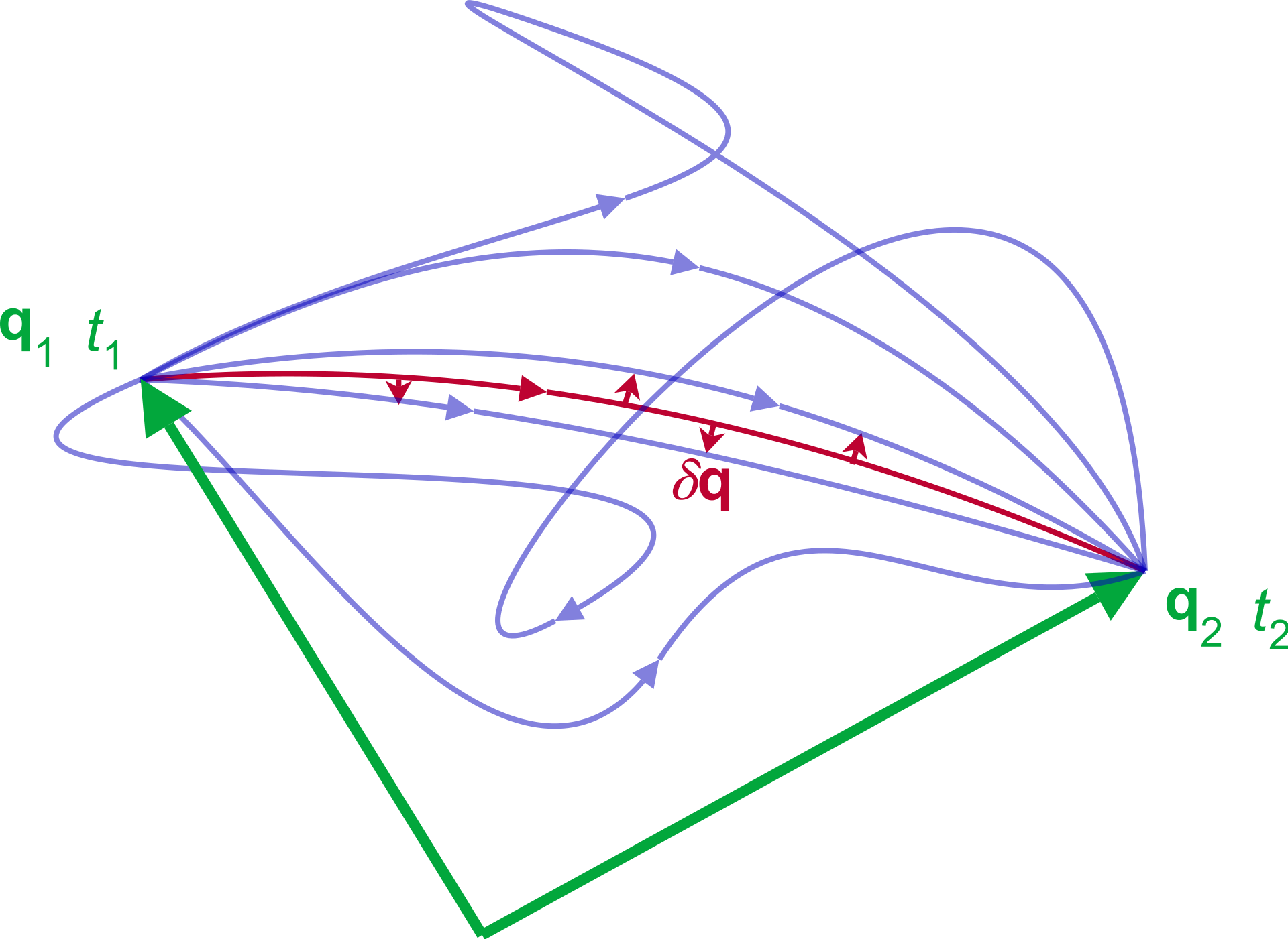
Figure 2.1: Principle of least action: As the system evolves, q traces a path through configuration space (only some are shown). The path taken by the system (red) has a stationary action under small changes in the configuration of the system.

Example 2.2 Let’s apply the Lagrangian mechanics formulas to the same problem as in the previous Example.

The expression of the kinetic energy, the potential energy, and the Lagrangian for our system are:

\[\begin{equation} \begin{aligned} K &= \frac{1}{2}m\dot{x}^2 \\ V &= mGx \\ L &= K-V = \frac{1}{2}m\dot{x}^2 - mGx. \end{aligned} \end{equation}\]

To get the equation of motion using eq. (2.5), we need to first take the partial derivative of \(L\) with respect to \(x\) (right hand side):

\[\begin{equation} \frac{\partial L}{\partial x}=-mG, \end{equation}\]

and then we need the derivative with respect to \(t\) of the derivative of the Lagrangian with respect to \(\dot{x}\) at the left hand side:

\[\begin{equation} \frac{d}{dt}\frac{\partial L}{\partial \dot{x}} = \frac{d\left(\frac{1}{2}m\dot{x}^2 - mGx\right)}{dt}= m\ddot{x}. \end{equation}\]

Putting this together, we get:

\[\begin{equation} \begin{aligned} m\ddot{x}&=-mG \\ \ddot{x} &= -G \\ \end{aligned} \end{equation}\]

Which is the same result as obtained from the Newtonian method. Integrating twice, we get the exact same formulas that we can use the same way.

The advantage of Lagrangian mechanics is that it is not constrained to use a coordinate system. For example, if we have a bead moving along a wire, we can define the coordinate system as the distance along the wire, making the formulas much simpler than in Newtonian mechanics. Also, since the Lagrangian depends on kinetic and potential energy it does a much better job with constraint forces.

2.1.3 Hamiltonian mechanics

A third way of obtaining the equation of motion is Hamiltonian mechanics, which uses the generalized momentum in place of velocity as a coordinate. The generalized momentum, \(\mathbf{p}\), is defined in terms of the Lagrangian and the coordinates \((\mathbf{r},\dot{\mathbf{r}})\):

\[\begin{equation} \mathbf{p} = \frac{\partial L}{\partial\dot{\mathbf{r}}}. \tag{2.6} \end{equation}\]

The Hamiltonian is defined from the Lagrangian by applying a Legendre transformation as:⁹

\[\begin{equation} H(\mathbf{p},\mathbf{r}) = \mathbf{p}\dot{\mathbf{r}} - L(\mathbf{r},\dot{\mathbf{r}}), \tag{2.7} \end{equation}\]

The Lagrangian equation of motion becomes a pair of equations known as the Hamiltonian system of equations:

\[\begin{equation} \begin{aligned} \dot{\mathbf{p}}=\frac{d\mathbf{p}}{dt} &= -\frac{\partial H}{\partial \mathbf{r}} \\ \dot{\mathbf{r}}=\frac{d\mathbf{r}}{dt} &= +\frac{\partial H}{\partial \mathbf{p}}, \end{aligned} \tag{2.8} \end{equation}\]

where \(H=H(\mathbf{p},\mathbf{r},t)\) is the Hamiltonian of the system, which often corresponds to its total energy. For a closed system, it is the sum of the kinetic and potential energy in the system:

\[\begin{equation} H = K + V. \tag{2.9} \end{equation}\]

Notice the difference between the Hamiltonian, eq. (2.9), and the Lagrangian, eq. (2.2). In Newtonian mechanics, the time evolution is obtained by computing the total force being exerted on each particle of the system, and from Newton’s second law, the time evolution of both position and velocity are computed. In contrast, in Hamiltonian mechanics, the time evolution is obtained by computing the Hamiltonian of the system in the generalized momenta and inserting it into Hamilton’s equations. This approach is equivalent to the one used in Lagrangian mechanics, since the Hamiltonian is the Legendre transform of the Lagrangian. The main motivation to use Hamiltonian mechanics instead of Lagrangian mechanics comes from the more simple description of complex dynamic systems.

Example 2.3 Let’s apply the Hamiltonian mechanics formulas to the same problem in the previous examples.

Using eq. (2.7), the Hamiltonian can be written as:

\[\begin{equation} H = m\dot{\mathbf{r}}\dot{\mathbf{r}} - \frac{1}{2}m\dot{\mathbf{r}}^2+mG\mathbf{r} = \frac{1}{2}m\dot{\mathbf{r}}^2+mG\mathbf{r}. \tag{2.10} \end{equation}\]

Since the Hamiltonian really depends on position and momentum, we need to get this in terms of \(\mathbf{r}\) and \(\mathbf{p}\), with \(\mathbf{r}=x\) and \(\mathbf{p} = p = m\dot{x}\) for our 1-dimensional system.¹⁰ Hence we have:

\[\begin{equation} H=\frac{p^2}{2m}+mGx, \end{equation}\]

from which we can use eqs. (2.8) to get:

\[\begin{equation} \begin{aligned} \dot{x} &= \frac{\partial H}{\partial p} = \frac{p}{m} \\ \dot{p} &=-\frac{\partial H}{\partial x} = -mG. \end{aligned} \end{equation}\]

These equations represent a major difference of the Hamiltonian method, since we describe the system using two first-order differential equations, rather than one second-order differential equation. In order to get the equation of motion, we need to take the derivative of \(\dot{x}\):

\[\begin{equation} \ddot{x} = \frac{d}{dt} \left( \frac{p}{m} \right) = \frac{\dot{p}}{m}, \end{equation}\]

and then replacing the definition of \(\dot{p}\) obtained above, we get:

\[\begin{equation} \ddot{x} = \frac{-mG}{m} = -G \end{equation}\]

which—once again—is the same result obtained for the two previous cases. Integrating this twice, we get the familiar equation of motion for our problem.

2.2 Coulomb’s Law

Coulomb’s Law states that the magnitude of the electrostatic force of attraction or repulsion between two point charges is directly proportional to the product of the magnitudes of charges and inversely proportional to the square of the distance between them:

\[\begin{equation} |\mathbf{F}| = k_e \frac{|q_1q_2|}{r^2} = \frac{1}{4\pi\varepsilon_0}\frac{|q_1q_2|}{r^{2}}. \tag{2.11} \end{equation}\]

The constant \(k_e\) is called the Coulomb constant and is equal to \({1}/{4\pi\varepsilon_0}\), where \(\varepsilon_0\) is the the vacuum permittivity constant; \(k_e \simeq 8.988\times10^9\;\mathrm{Nm^2C^{-2}}\). If the product \(q_1q_2\) is positive, the force between the two charges is repulsive; if the product is negative, the force between them is attractive.

2.2.1 Vector form of the Coulomb’s Law law

Coulomb’s law in vector form states that the electrostatic force \({\textstyle \mathbf {F}_{1}}\) experienced by a charge, \(q_{1}\) at position \(\mathbf {r}_{1}\), in the vicinity of another charge, \(q_{2}\) at position \(\mathbf {r}_{2}\), in a vacuum is equal \[\begin{equation} {\displaystyle \mathbf{F}_{1}={\frac {q_{1}q_{2}}{4\pi \varepsilon _{0}}}{\frac {\mathbf{r}_{1}-\mathbf{r}_{2}}{|\mathbf {r}_{1}-\mathbf{r}_{2}|^{3}}}={\frac {q_{1}q_{2}}{4\pi \varepsilon_{0}}}{\frac{\mathbf{\hat{r}} _{12}}{|\mathbf {r} _{12}|^{2}}}}, \tag{2.12} \end{equation}\]

where \({\textstyle {\boldsymbol {r}}_{12}={\boldsymbol {r}}_{1}-{\boldsymbol {r}}_{2}}\) is the vectorial distance between the charges, \({\textstyle {\widehat {\mathbf {r} }}_{12}={\frac {\mathbf {r} _{12}}{|\mathbf {r} _{12}|}}}\) a unit vector pointing from \({\textstyle q_{2}}\) to \({\textstyle q_{1}}\), and \(\varepsilon_{0}\) the vacuum permittivity constant. Here, \({\textstyle \mathbf {\hat {r}} _{12}}\) is used for the vector notation.

The vector form of Coulomb’s law is simply the scalar definition of the law with the direction given by the unit vector, \({\textstyle {\widehat {\mathbf {r} }}_{12}}\), parallel with the line from charge \(q_{2}\) to charge \(q_{1}\). If both charges have the same sign (like charges) then the product \(q_1q_2\) is positive and the direction of the force on \(q_{1}\) is given by \({\textstyle {\widehat {\mathbf {r} }}_{12}}\); the charges repel each other. If the charges have opposite signs then the product \(q_1q_2\) is negative and the direction of the force on \(q_{1}\) is \({\textstyle -{\hat {\mathbf {r} }}_{12}}\); the charges attract each other.

The electrostatic force \({\textstyle \mathbf {F} _{2}}\) experienced by \(q_{2}\), according to Newton’s third law, is \({\textstyle \mathbf {F} _{2}=-\mathbf {F} _{1}}\).

2.2.2 Electric field

An electric field is a vector field that associates to each point in space the Coulomb force experienced by a unit test charge. The strength and direction of the Coulomb force \({\textstyle \mathbf {F} }\) on a charge \({\textstyle q_{t}}\) depends on the electric field \({\textstyle \mathbf {E} }\) established by other charges that it finds itself in, such that \({\textstyle \mathbf {F} =q_{t}\mathbf {E} }\). In the simplest case, the field is considered to be generated solely by a single source point charge. If the field is generated by a positive source point charge \({\textstyle q}\), the direction of the electric field points along lines directed radially outwards from it, i.e. in the direction that a positive point test charge \({\textstyle q_{t}}\) would move if placed in the field. For a negative point source charge, the direction is radially inwards.

The magnitude of the electric field, \(|\mathbf{E}|\), can be derived from Coulomb’s law, eq. (2.11), by choosing one of the point charges to be the source (\(q_1=q\)), and the other to be the test charge (\(q_2=q_t\)), and is given by:

\[\begin{equation} {\displaystyle |\mathbf {E} |=|\mathbf{F}|\cdot \frac{1}{q_t}=\frac{1}{4\pi\varepsilon_0}{\frac {|q|}{r^{2}}}} \tag{2.13} \end{equation}\]

2.2.3 Electric Potential Energy

The electric potential energy of a system of point charges is defined as the work required to assemble this system of charges by bringing them close together, as in the system from an infinite distance.

The electrostatic potential energy, \(E\), of one point charge \(q\) at position \(\mathbf{r}\) in the presence of an electric field \(\mathbf{E}\) is defined as the negative of the work \(W\) done by the electrostatic force to bring it from a reference position at infinite distance \(\mathbf{r}_{\infty}\) to that position \(\mathbf{r}\):

\[\begin{equation} {\displaystyle E=-W_{\mathbf{r}_{\infty}\rightarrow \mathbf{r}}=-\int _{{\mathbf {r}}_{\infty}}^{\mathbf {r} }q\mathbf {E} (\mathbf {r'} )\cdot d \mathbf {r'} }, \tag{2.14} \end{equation}\]

where \(\mathbf{E}\) is the electrostatic field and \(d\mathbf{r'}\) is the displacement vector in a curve from the reference position \(\mathbf{r}_{\infty}\) to the final position \(\mathbf{r}\).

In the simplest case of two point charges \(q_1\) and \(q_2\), the electrostatic potential energy at position \(r\), can be derived from Coulomb’s Law, eq. (2.11), as:

\[\begin{equation} {\displaystyle E=|\mathbf{F}|\cdot r = {\frac{1}{4\pi\varepsilon_0}}{\frac{q_1q_2}{r}}}. \tag{2.15} \end{equation}\]

This last equation will become very important in future chapters. Notice the difference between eq. (2.15) for the energy, \(E\), and eq. (2.13) for the magnitude of the electric field, \(|\mathbf{E}|\).

---

3. Notice that \(\mathbf{r}\) \(\in\) \(\mathbb{R}^{3}\) is the position vector and \(\dot{\mathbf{r}}\) \(\in\) \(\mathbb{R}^{3}\) is the velocity vector. As such, all the equation of classical mechanics are vector equation in 3-dimensional space, and not just simple numerical equation. To simplify the picture, we can restrict ourselves to a 1-dimensional space, replace \(\mathbf{r}\) with \(x\), and forget the complications of vector algebra, as we do in the examples.↩︎

4. This example is based on Rhett Allain’s blog post that can be found (here)[https://rhettallain.com/2018/10/31/classical-mechanics-newtonian-lagrangian-and-hamiltonian/] ↩︎

5. Can you write a python program to do this calculation?↩︎

6. Sometimes also called principle of stationary action, or variational principle, or Hamilton’s principle.↩︎

7. This diagram is taken from Wikipedia by user Maschen, and distributed under CC0 license↩︎

8. The mathematical derivation of the Euler—Lagrange equaiton is rather long and unimportant at this stage. For the curious, it can be found here.↩︎

9. We have already encountered Legendre transform in The Live Textbook of Physical Chemistry 1 when transforming from the thermodynamic energy to any of the other thermodynamic potentials.↩︎

10. These equations are not universally valid, since they depend on the choice of coordinate system.↩︎